Chapter 1 Multilevel/Hierarchical Linear Modeling
1.2 What is Multilevel Modeling?
Multilevel modeling, also known as hierarchical linear modeling (HLM), mixed-effects modeling, or nested data analysis, is a statistical technique designed to analyze data that has a nested or hierarchical structure. This method acknowledges that observations are not always independent - a fundamental assumption of traditional regression analysis that is often violated in behavioral science research.
1.3 Core Concepts and Terminology
1.3.1 Hierarchical Data Structure
In multilevel modeling, data is organized in levels or hierarchies:
- Level 1 (Individual Level): The lowest level units (e.g., students, patients, measurements)
- Level 2 (Group Level): Higher level units that contain Level 1 units (e.g., classrooms, therapists, families)
- Level 3 (Organizational Level): Even higher level units (e.g., schools, hospitals, communities)
1.4 When to Use Multilevel Modeling
1.4.1 Research Questions That Require Multilevel Analysis:
- Nested Data Structure: When your data naturally clusters into groups
- Example: Student achievement scores nested within classrooms within schools
- Example: Patient outcomes nested within therapists within clinics
- Group-Level Effects: When you want to understand both individual and group influences
- Example: How does individual therapy engagement AND therapist experience affect treatment outcomes?
- Example: How do student motivation AND classroom climate affect academic performance?
- Cross-Level Interactions: When group-level variables moderate individual-level relationships
- Example: Does the relationship between anxiety and performance vary by school type?
- Example: Does the effect of medication vary by clinic setting?
1.4.2 Real-World Applications in Behavioral Science:
1.4.2.1 Educational Psychology:
- Question: “Do teaching methods affect student learning differently across schools?”
- Structure: Students (Level 1) nested in classrooms (Level 2) nested in schools (Level 3)
- Analysis: Examine how individual student characteristics and classroom/school factors influence learning outcomes
1.4.2.2 Clinical Psychology:
- Question: “How does therapist training influence the effectiveness of cognitive-behavioral therapy?”
- Structure: Therapy sessions (Level 1) nested in patients (Level 2) nested in therapists (Level 3)
- Analysis: Investigate patient progress while accounting for therapist effects
1.4.2.3 Organizational Psychology:
- Question: “How do individual personality traits and team culture interact to predict job satisfaction?”
- Structure: Employees (Level 1) nested in teams (Level 2) nested in organizations (Level 3)
- Analysis: Examine both individual and team-level predictors of satisfaction
1.5 Advantages of Multilevel Modeling
1.5.1 Statistical Benefits:
- Corrects for Dependency: Properly handles non-independence in nested data
- Prevents Type I Error: Avoids inflated significance tests that occur when ignoring clustering
- Increased Power: More efficient than analyzing groups separately
- Handles Missing Data: Can include all cases even with incomplete group membership
1.5.2 Substantive Benefits:
- Realistic Modeling: Reflects the natural structure of social and behavioral phenomena
- Cross-Level Questions: Allows investigation of how context influences individual outcomes
- Group Comparisons: Enables comparison of group effects while controlling for composition
- Policy Implications: Identifies whether interventions should target individuals or groups
1.6 When NOT to Use Multilevel Modeling
1.6.1 Inappropriate Situations:
- Small Number of Groups: Generally need at least 10-20 groups for reliable estimates
- No Theoretical Nesting: When grouping is arbitrary or theoretically meaningless
- No Group-Level Variance: When ICC is very low (< 0.05), simple regression may suffice
- Insufficient Group Size: When most groups have very few observations
1.7 Types of Multilevel Models
1.7.1 1. Random Intercept Model
- Allows group means to vary
- Assumes parallel slopes across groups
- Use when: Groups differ in baseline levels but relationships are consistent
1.8 Research Questions Addressed by Multilevel Modeling
1.8.1 1. Contextual Effects
- Question: “How does school poverty level affect student achievement beyond individual family income?”
- Analysis: Compare individual-level income effects with school-level poverty effects
1.8.2 2. Compositional Effects
- Question: “Does being in a class with high-achieving peers improve individual performance?”
- Analysis: Include both individual ability and class average ability as predictors
1.9 How to Report Multilevel Results in APA Format
1.9.1 Model Building Section:
“A series of multilevel models were fitted using maximum likelihood estimation. Model building followed a systematic approach, beginning with an unconditional model to estimate the intraclass correlation coefficient (ICC), followed by addition of Level 1 predictors, Level 2 predictors, and cross-level interactions.”
1.9.2 ICC Reporting:
“The unconditional model revealed significant between-group variance, ICC = .23, indicating that 23% of the variance in [outcome variable] was attributable to differences between [groups].”
1.10 Comprehensive APA Reporting Guide for Multilevel Modeling
1.10.1 Method Section Template
1.10.1.1 Participants and Design
“Participants included [N] patients nested within [N] therapists from [N] clinical settings. The multilevel structure was characterized by patients (Level 1, n = [N]) nested within therapists (Level 2, n = [N]), with an average of [M] patients per therapist (range: [min-max]).”
1.10.1.2 Statistical Analysis Plan
“Data were analyzed using multilevel modeling to account for the nested structure of patients within therapists. Model building followed a systematic approach: (1) unconditional model to calculate intraclass correlation, (2) random intercept model with Level 1 predictors, (3) random slope model allowing treatment effects to vary by therapist, and (4) full model including Level 2 therapist characteristics.”
“Models were fitted using maximum likelihood estimation in R using the lme4 package. Model comparisons were conducted using likelihood ratio tests. Statistical significance was evaluated at α = .05.”
1.10.2 Results Section Template
1.10.2.1 Preliminary Analysis
“Preliminary analysis revealed that [X]% of the variance in post-treatment depression scores was attributable to between-therapist differences (ICC = .XX, 95% CI [.XX, .XX]), justifying the use of multilevel modeling.”
1.10.2.2 Model Building Results
“Model building proceeded systematically. The addition of Level 1 predictors significantly improved model fit compared to the unconditional model, χ²(3) = XX.XX, p < .001. The random slope model, allowing treatment duration effects to vary across therapists, provided further improvement, χ²(2) = XX.XX, p < .05. The final model, including therapist-level predictors, demonstrated the best fit, χ²(2) = XX.XX, p < .01.”
1.10.2.3 Fixed Effects Results
“Fixed effects analysis revealed several significant predictors of post-treatment depression scores (see Table X). Higher baseline depression severity was associated with higher post-treatment scores (b = X.XX, SE = X.XX, t = X.XX, p < .001, 95% CI [X.XX, X.XX]). Treatment duration showed a protective effect (b = -X.XX, SE = X.XX, t = -X.XX, p < .001, 95% CI [-X.XX, -X.XX]), with each additional week of treatment associated with a X.XX-point reduction in depression scores.”
“At the therapist level, experience significantly predicted better patient outcomes (b = -X.XX, SE = X.XX, t = -X.XX, p < .01, 95% CI [-X.XX, -X.XX]). Compared to humanistic therapy, CBT was associated with significantly lower post-treatment depression scores (b = -X.XX, SE = X.XX, t = -X.XX, p < .001, 95% CI [-X.XX, -X.XX]).”
1.10.2.4 Random Effects Results
“Random effects analysis indicated significant variability in both intercepts (τ₀₀ = X.XX, p < .001) and slopes for treatment duration across therapists (τ₁₁ = X.XX, p < .05). This suggests that therapists differed in both their baseline effectiveness and their ability to utilize extended treatment duration.”
1.10.2.5 Effect Sizes and Clinical Significance
“Effect sizes were calculated using Cohen’s guidelines for multilevel models. The effect of CBT (d = X.XX) represents a medium effect size, while therapist experience (d = X.XX) shows a small to medium effect. The model explained XX% of Level 1 variance and XX% of Level 2 variance.”
1.10.3 Tables and Figures
1.10.3.1 Table 1: Descriptive Statistics and Correlations
[Include means, SDs, and correlations for all variables, separately by level when appropriate]
1.10.3.2 Table 2: Model Comparison Statistics
[Include fit statistics for each model: -2LL, AIC, BIC, χ² difference tests]
1.10.4 Discussion Template
1.10.4.1 Interpretation
“Results support a multilevel perspective on therapy effectiveness, with significant effects observed at both patient and therapist levels. The ICC of .XX indicates that [interpretation of practical significance]. The significant random slope variance suggests that the relationship between treatment duration and outcomes varies meaningfully across therapists.”
1.10.4.2 Clinical Implications
“Findings suggest that [specific clinical recommendations based on results]. The therapist-level effects highlight the importance of [training/supervision/approach implications]. The random slope findings indicate that [personalization/matching implications].”
1.10.4.3 Limitations
“Several limitations should be noted. First, the observational design limits causal inference. Second, therapist selection may have influenced results. Third, unmeasured therapist characteristics may explain additional variance.”
1.10.4.4 Future Directions
“Future research should examine [specific recommendations]. Cross-level interactions between patient and therapist characteristics warrant investigation. Longitudinal growth models could illuminate treatment trajectories.”
This comprehensive approach to reporting multilevel results ensures transparency, replicability, and appropriate interpretation of complex hierarchical data structures common in behavioral science research.
1.11 Mathematical Foundation
The basic multilevel model can be expressed as:
Level 1 (Individual level): \[Y_{ij} = \beta_{0j} + \beta_{1j}X_{ij} + r_{ij}\]
Level 2 (Group level): \[\beta_{0j} = \gamma_{00} + \gamma_{01}W_j + u_{0j}\] \[\beta_{1j} = \gamma_{10} + \gamma_{11}W_j + u_{1j}\]
Where: - \(Y_{ij}\) is the outcome for individual \(i\) in group \(j\) - \(X_{ij}\) is a level-1 predictor - \(W_j\) is a level-2 predictor - \(r_{ij}\) is the level-1 residual - \(u_{0j}\) and \(u_{1j}\) are level-2 residuals
1.12 Required Packages
# Set CRAN mirror
options(repos = c(CRAN = "https://cran.rstudio.com/"))

# Install packages if not already installed
if (!require("lme4")) install.packages("lme4")
if (!require("lmerTest")) install.packages("lmerTest")
if (!require("report")) install.packages("report")
if (!require("ggplot2")) install.packages("ggplot2")
if (!require("dplyr")) install.packages("dplyr")
if (!require("performance")) install.packages("performance")
if (!require("see")) install.packages("see")
if (!require("sjPlot")) install.packages("sjPlot")
if (!require("ggeffects")) install.packages("ggeffects")

library(lme4)
library(lmerTest)
library(report)
library(ggplot2)
library(dplyr)
library(performance)
library(see)
library(sjPlot)
library(ggeffects)
1.13 Step-by-Step Guide to Multilevel Analysis
1.13.1 Overview of the Analysis Process
This tutorial demonstrates multilevel modeling using a realistic clinical psychology scenario. We will:
- Simulate realistic nested data representing patients nested within therapists
- Build models progressively from simple to complex
- Interpret results with clinical significance in mind
- Report findings using APA format guidelines
1.13.2 Why This Example is Important
In clinical psychology, ignoring the therapist effect can lead to: - Inflated Type I error rates: Treating patients as independent when they share therapists - Incorrect confidence intervals: Underestimating uncertainty in treatment effects - Missed insights: Failing to identify therapist characteristics that enhance treatment - Poor generalizability: Results may not apply to different clinical settings
1.14 Data Simulation: Therapy Effectiveness Study
1.14.1 Study Design Explanation
We are simulating a study examining cognitive-behavioral therapy (CBT) effectiveness for depression, where:
- Research Question: “How do patient characteristics and therapist factors influence depression treatment outcomes?”
- Design: Patients (Level 1) nested within therapists (Level 2)
- Outcome: Depression score change from baseline to 12-week follow-up
- Level 1 Predictors: Patient age, baseline severity, therapy adherence
- Level 2 Predictors: Therapist experience, therapy approach (CBT vs. other)
1.14.2 Why This Design Requires Multilevel Modeling
- Non-independence: Patients seeing the same therapist are more similar than patients seeing different therapists
- Therapist effects: Some therapists may be more effective regardless of patient characteristics
- Cross-level interactions: Therapist experience might moderate the relationship between patient adherence and outcomes
set.seed(123)

# Number of therapists and patients per therapist
n_therapists <- 20
n_patients_per_therapist <- 15
n_total <- n_therapists * n_patients_per_therapist

# Create therapist-level data
therapist_data <- data.frame(
  therapist_id = 1:n_therapists,
  therapist_experience = rnorm(n_therapists, mean = 5, sd = 2), # Years of experience
  therapy_approach = sample(c("CBT", "Psychodynamic", "Humanistic"), n_therapists, replace = TRUE)
)

# Create patient-level data
patient_data <- data.frame(
  patient_id = 1:n_total,
  therapist_id = rep(1:n_therapists, each = n_patients_per_therapist),
  age = rnorm(n_total, mean = 35, sd = 12),
  baseline_depression = rnorm(n_total, mean = 20, sd = 5),
  treatment_weeks = sample(8:16, n_total, replace = TRUE)
)

# Merge data
full_data <- merge(patient_data, therapist_data, by = "therapist_id")

# Generate outcome variable with multilevel structure
# Therapist random effects
therapist_effects <- rnorm(n_therapists, mean = 0, sd = 2)
full_data$therapist_effect <- therapist_effects[full_data$therapist_id]

# Generate post-treatment depression scores
full_data$post_depression <- with(full_data,
  15 + # Intercept
  0.3 * baseline_depression + # Baseline effect
  -0.5 * treatment_weeks + # Treatment effect
  -1.2 * therapist_experience + # Therapist experience effect
  ifelse(therapy_approach == "CBT", -2, ifelse(therapy_approach == "Psychodynamic", -1, 0)) + # Approach effect
  therapist_effect + # Random therapist effect
  rnorm(n_total, mean = 0, sd = 3) # Individual residual
)

# Create categorical variables
full_data$therapy_approach <- as.factor(full_data$therapy_approach)
full_data$therapist_id <- as.factor(full_data$therapist_id)

# Display first few rows
head(full_data, 10)
## therapist_id patient_id age baseline_depression treatment_weeks
## 1 1 1 33.447072 12.80081 16
## 2 1 2 45.640834 14.96917 12
## 3 1 3 33.183248 15.29822 8
## 4 1 4 38.957494 20.26726 16
## 5 1 5 -3.727874 17.13027 16
## 6 1 6 25.738499 21.10274 14
## 7 1 7 38.438583 15.82742 9
## 8 1 8 20.353856 19.34823 15
## 9 1 9 40.214605 22.83665 14
## 10 1 10 44.602122 26.04233 13
## therapist_experience therapy_approach therapist_effect post_depression
## 1 3.879049 Humanistic 0.09261415 4.666771
## 2 3.879049 Humanistic 0.09261415 12.080897
## 3 3.879049 Humanistic 0.09261415 6.629754
## 4 3.879049 Humanistic 0.09261415 9.120385
## 5 3.879049 Humanistic 0.09261415 6.300653
## 6 3.879049 Humanistic 0.09261415 14.396872
## 7 3.879049 Humanistic 0.09261415 12.188104
## 8 3.879049 Humanistic 0.09261415 12.071650
## 9 3.879049 Humanistic 0.09261415 8.005024
## 10 3.879049 Humanistic 0.09261415 15.3718041.15 Exploratory Data Analysis
# Summary statistics
summary(full_data[, c("post_depression", "baseline_depression", "treatment_weeks", "therapist_experience")])
## post_depression baseline_depression treatment_weeks therapist_experience
## Min. :-10.632 Min. : 4.765 Min. : 8.00 Min. :1.067
## 1st Qu.: 3.590 1st Qu.:16.199 1st Qu.:10.00 1st Qu.:4.013
## Median : 7.449 Median :19.740 Median :12.00 Median :5.240
## Mean : 7.177 Mean :19.446 Mean :11.96 Mean :5.283
## 3rd Qu.: 11.013 3rd Qu.:22.819 3rd Qu.:14.00 3rd Qu.:6.097
## Max. : 19.700 Max. :35.286 Max. :16.00 Max. :8.574# Visualize the multilevel structure
ggplot(full_data, aes(x = treatment_weeks, y = post_depression, color = therapy_approach)) +
geom_point(alpha = 0.6) +
geom_smooth(method = "lm", se = FALSE) +
facet_wrap(~ therapist_id, ncol = 5) +
labs(title = "Post-Treatment Depression by Treatment Weeks",
subtitle = "Separated by Therapist (showing multilevel structure)",
x = "Treatment Weeks",
y = "Post-Treatment Depression Score") +
theme_minimal() +
theme(legend.position = "bottom")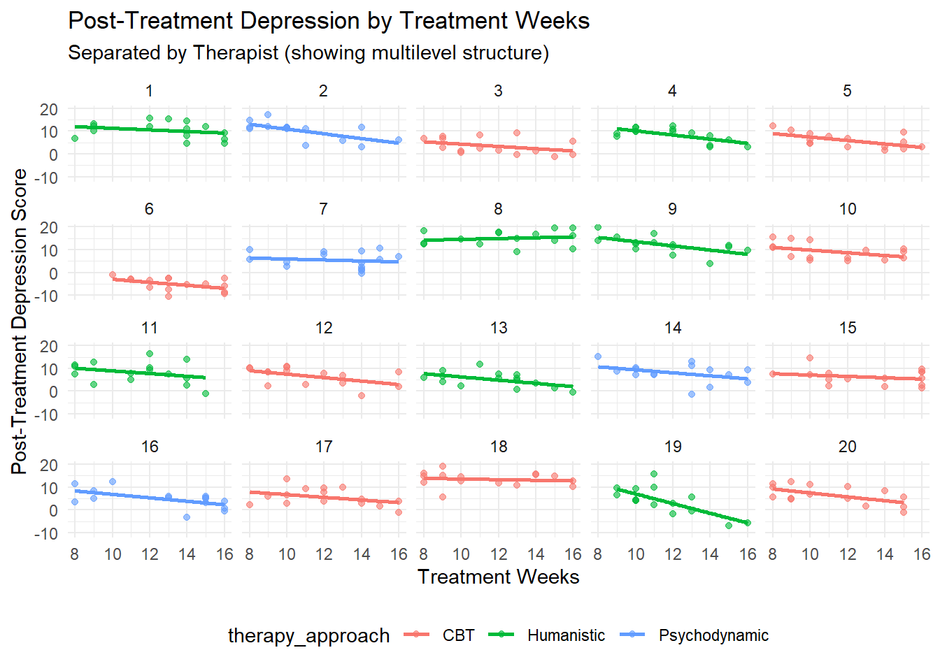
# Intraclass correlation visualization
ggplot(full_data, aes(x = factor(therapist_id), y = post_depression, fill = therapy_approach)) +
  geom_boxplot(alpha = 0.7) +
  labs(title = "Depression Scores by Therapist",
       x = "Therapist ID",
       y = "Post-Treatment Depression Score") +
  theme_minimal() +
  theme(axis.text.x = element_text(angle = 45, hjust = 1))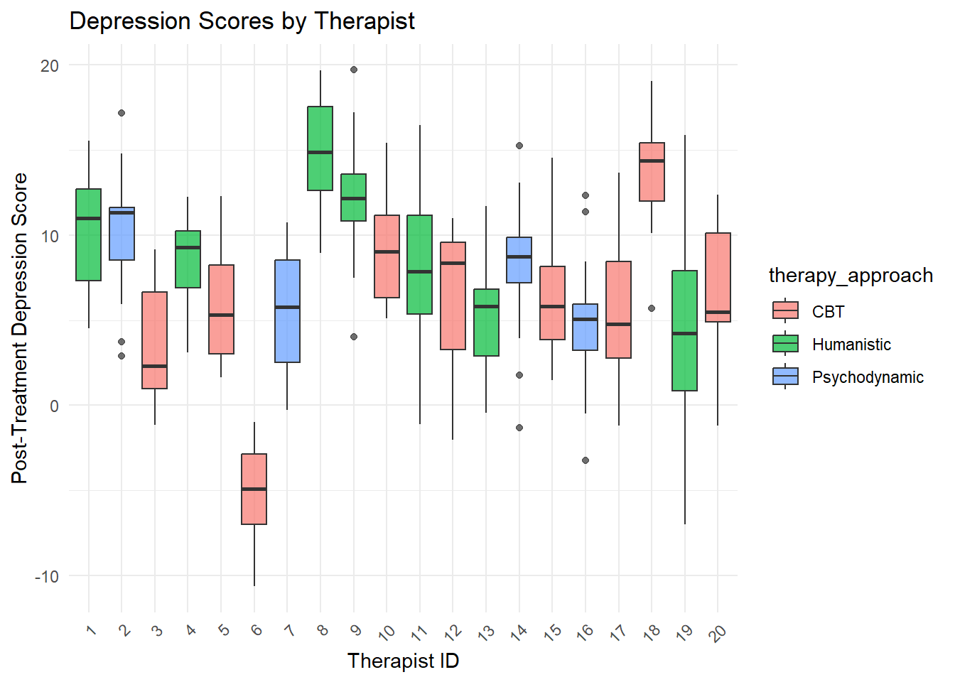
1.16 Multilevel Model Analysis: Progressive Model Building
1.16.1 The Model Building Strategy
Multilevel modeling follows a systematic approach to build complexity gradually:
- Null Model: Establishes baseline and calculates ICC
- Random Intercept: Adds Level 1 predictors while allowing group intercepts to vary
- Random Slope: Allows slopes to vary across groups
- Cross-Level Interaction: Tests how group variables moderate individual relationships
This progression helps identify the most appropriate model complexity and provides insights at each step.
1.16.2 Step 1: Null Model (Unconditional/Intercept-Only Model)
1.16.2.1 Purpose and Interpretation
The null model answers: “How much variance exists between therapists before accounting for any predictors?”
This model: - Contains no predictors (unconditional) - Estimates overall mean outcome across all patients - Partitions variance into within-therapist and between-therapist components - Calculates the Intraclass Correlation Coefficient (ICC)
1.16.2.2 Clinical Significance
- High ICC (> .10): Strong therapist effects - multilevel modeling essential
- Low ICC (< .05): Weak therapist effects - simple regression may suffice
- Moderate ICC (.05-.10): Some therapist effects - multilevel modeling recommended
1.16.2.3 APA Reporting for Null Model
“An unconditional multilevel model was fitted to examine the extent of between-therapist variability in post-treatment depression scores. The model partitioned variance into within-therapist (Level 1) and between-therapist (Level 2) components.”
# Null model to calculate ICC
# Formula: outcome ~ 1 + (1 | grouping_variable)
# Translation: "Model the outcome with only an intercept, allowing intercepts to vary by therapist"
null_model <- lmer(post_depression ~ 1 + (1 | therapist_id), data = full_data)
summary(null_model)
## Linear mixed model fit by REML. t-tests use Satterthwaite's method [
## lmerModLmerTest]
## Formula: post_depression ~ 1 + (1 | therapist_id)
## Data: full_data
##
## REML criterion at convergence: 1711.1
##
## Scaled residuals:
## Min 1Q Median 3Q Max
## -2.91260 -0.69829 0.05929 0.59160 3.07259
##
## Random effects:
## Groups Name Variance Std.Dev.
## therapist_id (Intercept) 17.33 4.163
## Residual 14.57 3.817
## Number of obs: 300, groups: therapist_id, 20
##
## Fixed effects:
## Estimate Std. Error df t value Pr(>|t|)
## (Intercept) 7.1774 0.9566 19.0000 7.503 4.28e-07 ***
## ---
## Signif. codes: 0 '***' 0.001 '**' 0.01 '*' 0.05 '.' 0.1 ' ' 1# Calculate Intraclass Correlation Coefficient (ICC)
icc_result <- performance::icc(null_model)
print(icc_result)## # Intraclass Correlation Coefficient
##
## Adjusted ICC: 0.543
## Unadjusted ICC: 0.543# Manual ICC calculation for understanding
variance_components <- VarCorr(null_model)
between_therapist_var <- as.numeric(variance_components$therapist_id[1])
within_therapist_var <- attr(variance_components, "sc")^2
icc_manual <- between_therapist_var / (between_therapist_var + within_therapist_var)
cat("Manual ICC calculation:", round(icc_manual, 3), "\n")## Manual ICC calculation: 0.5431.16.3 Step 2: Random Intercept Model with Level 1 Predictors
1.16.3.1 Purpose and Interpretation
This model answers: “How do patient characteristics predict outcomes, while accounting for therapist differences?”
This model: - Adds individual-level (Level 1) predictors - Maintains random intercepts (therapists can have different baseline effectiveness) - Assumes slopes are the same across therapists (parallel regression lines) - Shows how much Level 1 predictors explain within-therapist variance
1.16.3.2 What Each Predictor Tells Us
- Baseline Depression: Controls for initial severity (essential covariate)
- Treatment Weeks: Captures dose-response relationship
- Age: Tests whether age influences treatment response
1.16.3.3 APA Reporting for Random Intercept Model
“A random intercept model was fitted including patient-level predictors (baseline depression severity, treatment duration, and age) while allowing therapist intercepts to vary randomly.”
# Random intercept model with level-1 predictors
# Formula: outcome ~ fixed_predictors + (1 | grouping_variable)
# Translation: "Model outcome using patient predictors, with therapist-specific intercepts"
model_1 <- lmer(post_depression ~ baseline_depression + treatment_weeks + age +
                (1 | therapist_id), data = full_data)
summary(model_1)
## Linear mixed model fit by REML. t-tests use Satterthwaite's method [
## lmerModLmerTest]
## Formula: post_depression ~ baseline_depression + treatment_weeks + age +
## (1 | therapist_id)
## Data: full_data
##
## REML criterion at convergence: 1602.8
##
## Scaled residuals:
## Min 1Q Median 3Q Max
## -2.49276 -0.64439 0.04738 0.63619 2.30326
##
## Random effects:
## Groups Name Variance Std.Dev.
## therapist_id (Intercept) 16.37 4.046
## Residual 9.54 3.089
## Number of obs: 300, groups: therapist_id, 20
##
## Fixed effects:
## Estimate Std. Error df t value Pr(>|t|)
## (Intercept) 6.809321 1.623484 138.757192 4.194 4.86e-05 ***
## baseline_depression 0.333862 0.038025 278.520388 8.780 < 2e-16 ***
## treatment_weeks -0.515446 0.072022 278.731405 -7.157 7.33e-12 ***
## age 0.001109 0.015146 278.204869 0.073 0.942
## ---
## Signif. codes: 0 '***' 0.001 '**' 0.01 '*' 0.05 '.' 0.1 ' ' 1
##
## Correlation of Fixed Effects:
## (Intr) bsln_d trtmn_
## bsln_dprssn -0.505
## tretmnt_wks -0.630 0.141
## age -0.348 -0.078 0.107## We fitted a linear mixed model (estimated using REML and nloptwrap optimizer)
## to predict post_depression with baseline_depression, treatment_weeks and age
## (formula: post_depression ~ baseline_depression + treatment_weeks + age). The
## model included therapist_id as random effect (formula: ~1 | therapist_id). The
## model's total explanatory power is substantial (conditional R2 = 0.69) and the
## part related to the fixed effects alone (marginal R2) is of 0.17. The model's
## intercept, corresponding to baseline_depression = 0, treatment_weeks = 0 and
## age = 0, is at 6.81 (95% CI [3.61, 10.00], t(294) = 4.19, p < .001). Within
## this model:
##
## - The effect of baseline depression is statistically significant and positive
## (beta = 0.33, 95% CI [0.26, 0.41], t(294) = 8.78, p < .001; Std. beta = 0.29,
## 95% CI [0.23, 0.36])
## - The effect of treatment weeks is statistically significant and negative (beta
## = -0.52, 95% CI [-0.66, -0.37], t(294) = -7.16, p < .001; Std. beta = -0.24,
## 95% CI [-0.31, -0.18])
## - The effect of age is statistically non-significant and positive (beta =
## 1.11e-03, 95% CI [-0.03, 0.03], t(294) = 0.07, p = 0.942; Std. beta = 2.43e-03,
## 95% CI [-0.06, 0.07])
##
## Standardized parameters were obtained by fitting the model on a standardized
## version of the dataset. 95% Confidence Intervals (CIs) and p-values were
## computed using a Wald t-distribution approximation.## Data: full_data
## Models:
## null_model: post_depression ~ 1 + (1 | therapist_id)
## model_1: post_depression ~ baseline_depression + treatment_weeks + age + (1 | therapist_id)
## npar AIC BIC logLik -2*log(L) Chisq Df Pr(>Chisq)
## null_model 3 1718.8 1729.9 -856.39 1712.8
## model_1 6 1601.7 1623.9 -794.85 1589.7 123.09 3 < 2.2e-16 ***
## ---
## Signif. codes: 0 '***' 0.001 '**' 0.01 '*' 0.05 '.' 0.1 ' ' 11.16.4 Step 3: Random Slope Model
1.16.4.1 Purpose and Interpretation
This model answers: “Do the effects of patient characteristics vary across therapists?”
This model: - Allows both intercepts AND slopes to vary by therapist - Tests whether treatment effectiveness differs across therapists - Shows if some therapists are better at working with certain types of patients - Requires sufficient data per group (typically 10+ observations per group)
1.16.4.2 When to Use Random Slopes
- Theoretical reason: You expect treatment effects to vary by context
- Statistical evidence: Likelihood ratio test favors random slope model
- Practical significance: Understanding therapist differences matters for training
1.16.4.3 Clinical Significance
If treatment weeks has varying slopes: - Some therapists may be more effective with longer treatment - Others may achieve results quickly - This suggests need for therapist-specific training or patient matching
1.16.4.4 APA Reporting for Random Slope Model
“A random slope model was fitted allowing the effect of treatment duration to vary across therapists, while controlling for patient baseline characteristics.”
# Random slope model allowing treatment effect to vary by therapist
# Formula: outcome ~ predictors + (1 + varying_predictor | grouping_variable)
# Translation: "Allow both intercepts and treatment_weeks slopes to vary by therapist"
model_2 <- lmer(post_depression ~ baseline_depression + treatment_weeks + age +
                (1 + treatment_weeks | therapist_id), data = full_data)
summary(model_2)
## Linear mixed model fit by REML. t-tests use Satterthwaite's method [
## lmerModLmerTest]
## Formula: post_depression ~ baseline_depression + treatment_weeks + age +
## (1 + treatment_weeks | therapist_id)
## Data: full_data
##
## REML criterion at convergence: 1598.4
##
## Scaled residuals:
## Min 1Q Median 3Q Max
## -2.53388 -0.67797 0.07469 0.63664 2.38443
##
## Random effects:
## Groups Name Variance Std.Dev. Corr
## therapist_id (Intercept) 5.80354 2.4091
## treatment_weeks 0.03846 0.1961 0.39
## Residual 9.33583 3.0555
## Number of obs: 300, groups: therapist_id, 20
##
## Fixed effects:
## Estimate Std. Error df t value Pr(>|t|)
## (Intercept) 7.223037 1.437992 55.429609 5.023 5.62e-06 ***
## baseline_depression 0.325298 0.037655 274.046928 8.639 4.78e-16 ***
## treatment_weeks -0.542454 0.083788 17.769485 -6.474 4.61e-06 ***
## age 0.003856 0.015048 275.358908 0.256 0.798
## ---
## Signif. codes: 0 '***' 0.001 '**' 0.01 '*' 0.05 '.' 0.1 ' ' 1
##
## Correlation of Fixed Effects:
## (Intr) bsln_d trtmn_
## bsln_dprssn -0.563
## tretmnt_wks -0.522 0.120
## age -0.386 -0.081 0.088## We fitted a linear mixed model (estimated using REML and nloptwrap optimizer)
## to predict post_depression with baseline_depression, treatment_weeks and age
## (formula: post_depression ~ baseline_depression + treatment_weeks + age). The
## model included treatment_weeks as random effects (formula: ~1 + treatment_weeks
## | therapist_id). The model's total explanatory power is substantial
## (conditional R2 = 0.69) and the part related to the fixed effects alone
## (marginal R2) is of 0.17. The model's intercept, corresponding to
## baseline_depression = 0, treatment_weeks = 0 and age = 0, is at 7.22 (95% CI
## [4.39, 10.05], t(292) = 5.02, p < .001). Within this model:
##
## - The effect of baseline depression is statistically significant and positive
## (beta = 0.33, 95% CI [0.25, 0.40], t(292) = 8.64, p < .001; Std. beta = 0.29,
## 95% CI [0.22, 0.35])
## - The effect of treatment weeks is statistically significant and negative (beta
## = -0.54, 95% CI [-0.71, -0.38], t(292) = -6.47, p < .001; Std. beta = -0.25,
## 95% CI [-0.33, -0.18])
## - The effect of age is statistically non-significant and positive (beta =
## 3.86e-03, 95% CI [-0.03, 0.03], t(292) = 0.26, p = 0.798; Std. beta = 8.46e-03,
## 95% CI [-0.06, 0.07])
##
## Standardized parameters were obtained by fitting the model on a standardized
## version of the dataset. 95% Confidence Intervals (CIs) and p-values were
## computed using a Wald t-distribution approximation.# Test if random slope is justified
anova(model_1, model_2) # Compare random intercept vs random slope## Data: full_data
## Models:
## model_1: post_depression ~ baseline_depression + treatment_weeks + age + (1 | therapist_id)
## model_2: post_depression ~ baseline_depression + treatment_weeks + age + (1 + treatment_weeks | therapist_id)
## npar AIC BIC logLik -2*log(L) Chisq Df Pr(>Chisq)
## model_1 6 1601.7 1623.9 -794.85 1589.7
## model_2 8 1601.3 1630.9 -792.64 1585.3 4.4217 2 0.10961.16.5 Step 4: Full Multilevel Model with Level 2 Predictors
1.16.5.1 Purpose and Interpretation
This model answers: “How do therapist characteristics influence patient outcomes?”
This model: - Adds therapist-level (Level 2) predictors - Tests cross-level effects (how therapist traits affect all their patients) - Maintains random slopes if justified - Provides complete picture of multilevel influences
1.16.5.2 Therapist-Level Predictors
- Therapist Experience: Tests whether experience improves outcomes
- Therapy Approach: Compares CBT effectiveness to other approaches
- Cross-level interactions: Could test if experience moderates treatment effects
1.16.5.3 Clinical Implications
- Experience effects: Informs training and supervision needs
- Approach effects: Guides evidence-based practice recommendations
- Random effects: Shows remaining therapist variability after accounting for measured characteristics
1.16.5.4 APA Reporting for Full Model
“The final model included both patient-level predictors (baseline severity, treatment duration, age) and therapist-level predictors (experience, therapeutic approach) while allowing treatment effects to vary randomly across therapists.”
# Full model with therapist-level predictors
# This tests both individual and contextual effects
model_3 <- lmer(post_depression ~ baseline_depression + treatment_weeks + age +
                therapist_experience + therapy_approach +
                (1 + treatment_weeks | therapist_id), data = full_data)
summary(model_3)
## Linear mixed model fit by REML. t-tests use Satterthwaite's method [
## lmerModLmerTest]
## Formula: post_depression ~ baseline_depression + treatment_weeks + age +
## therapist_experience + therapy_approach + (1 + treatment_weeks |
## therapist_id)
## Data: full_data
##
## REML criterion at convergence: 1568.8
##
## Scaled residuals:
## Min 1Q Median 3Q Max
## -2.56089 -0.66296 0.02251 0.64389 2.42560
##
## Random effects:
## Groups Name Variance Std.Dev. Corr
## therapist_id (Intercept) 1.63925 1.2803
## treatment_weeks 0.04602 0.2145 -0.62
## Residual 9.30176 3.0499
## Number of obs: 300, groups: therapist_id, 20
##
## Fixed effects:
## Estimate Std. Error df t value Pr(>|t|)
## (Intercept) 13.756597 1.802821 30.150096 7.631 1.59e-08
## baseline_depression 0.325485 0.037424 277.104598 8.697 3.06e-16
## treatment_weeks -0.553462 0.085809 17.712310 -6.450 4.91e-06
## age 0.002394 0.015000 277.351409 0.160 0.87329
## therapist_experience -1.513844 0.234682 13.149271 -6.451 2.05e-05
## therapy_approachHumanistic 2.969809 0.979146 13.369273 3.033 0.00935
## therapy_approachPsychodynamic 3.000868 1.189509 13.387146 2.523 0.02502
##
## (Intercept) ***
## baseline_depression ***
## treatment_weeks ***
## age
## therapist_experience ***
## therapy_approachHumanistic **
## therapy_approachPsychodynamic *
## ---
## Signif. codes: 0 '***' 0.001 '**' 0.01 '*' 0.05 '.' 0.1 ' ' 1
##
## Correlation of Fixed Effects:
## (Intr) bsln_d trtmn_ age thrps_ thrp_H
## bsln_dprssn -0.420
## tretmnt_wks -0.473 0.117
## age -0.298 -0.080 0.084
## thrpst_xprn -0.610 -0.038 -0.059 -0.014
## thrpy_pprcH -0.227 -0.012 -0.022 0.001 0.010
## thrpy_pprcP -0.080 0.011 0.006 0.010 -0.189 0.354## We fitted a linear mixed model (estimated using REML and nloptwrap optimizer)
## to predict post_depression with baseline_depression, treatment_weeks, age,
## therapist_experience and therapy_approach (formula: post_depression ~
## baseline_depression + treatment_weeks + age + therapist_experience +
## therapy_approach). The model included treatment_weeks as random effects
## (formula: ~1 + treatment_weeks | therapist_id). The model's total explanatory
## power is substantial (conditional R2 = 0.69) and the part related to the fixed
## effects alone (marginal R2) is of 0.54. The model's intercept, corresponding to
## baseline_depression = 0, treatment_weeks = 0, age = 0, therapist_experience = 0
## and therapy_approach = CBT, is at 13.76 (95% CI [10.21, 17.30], t(289) = 7.63,
## p < .001). Within this model:
##
## - The effect of baseline depression is statistically significant and positive
## (beta = 0.33, 95% CI [0.25, 0.40], t(289) = 8.70, p < .001; Std. beta = 0.29,
## 95% CI [0.22, 0.35])
## - The effect of treatment weeks is statistically significant and negative (beta
## = -0.55, 95% CI [-0.72, -0.38], t(289) = -6.45, p < .001; Std. beta = -0.26,
## 95% CI [-0.34, -0.18])
## - The effect of age is statistically non-significant and positive (beta =
## 2.39e-03, 95% CI [-0.03, 0.03], t(289) = 0.16, p = 0.873; Std. beta = 5.25e-03,
## 95% CI [-0.06, 0.07])
## - The effect of therapist experience is statistically significant and negative
## (beta = -1.51, 95% CI [-1.98, -1.05], t(289) = -6.45, p < .001; Std. beta =
## -0.52, 95% CI [-0.67, -0.36])
## - The effect of therapy approach [Humanistic] is statistically significant and
## positive (beta = 2.97, 95% CI [1.04, 4.90], t(289) = 3.03, p = 0.003; Std. beta
## = 0.53, 95% CI [0.19, 0.88])
## - The effect of therapy approach [Psychodynamic] is statistically significant
## and positive (beta = 3.00, 95% CI [0.66, 5.34], t(289) = 2.52, p = 0.012; Std.
## beta = 0.54, 95% CI [0.12, 0.96])
##
## Standardized parameters were obtained by fitting the model on a standardized
## version of the dataset. 95% Confidence Intervals (CIs) and p-values were
## computed using a Wald t-distribution approximation.## Data: full_data
## Models:
## model_2: post_depression ~ baseline_depression + treatment_weeks + age + (1 + treatment_weeks | therapist_id)
## model_3: post_depression ~ baseline_depression + treatment_weeks + age + therapist_experience + therapy_approach + (1 + treatment_weeks | therapist_id)
## npar AIC BIC logLik -2*log(L) Chisq Df Pr(>Chisq)
## model_2 8 1601.3 1630.9 -792.64 1585.3
## model_3 11 1578.7 1619.4 -778.35 1556.7 28.591 3 2.729e-06 ***
## ---
## Signif. codes: 0 '***' 0.001 '**' 0.01 '*' 0.05 '.' 0.1 ' ' 11.17 Model Comparison
# Compare models using AIC, BIC, and likelihood ratio tests
anova(null_model, model_1, model_2, model_3)
## Data: full_data
## Models:
## null_model: post_depression ~ 1 + (1 | therapist_id)
## model_1: post_depression ~ baseline_depression + treatment_weeks + age + (1 | therapist_id)
## model_2: post_depression ~ baseline_depression + treatment_weeks + age + (1 + treatment_weeks | therapist_id)
## model_3: post_depression ~ baseline_depression + treatment_weeks + age + therapist_experience + therapy_approach + (1 + treatment_weeks | therapist_id)
## npar AIC BIC logLik -2*log(L) Chisq Df Pr(>Chisq)
## null_model 3 1718.8 1729.9 -856.39 1712.8
## model_1 6 1601.7 1623.9 -794.85 1589.7 123.0858 3 < 2.2e-16 ***
## model_2 8 1601.3 1630.9 -792.64 1585.3 4.4217 2 0.1096
## model_3 11 1578.7 1619.4 -778.35 1556.7 28.5915 3 2.729e-06 ***
## ---
## Signif. codes: 0 '***' 0.001 '**' 0.01 '*' 0.05 '.' 0.1 ' ' 1## # Comparison of Model Performance Indices
##
## Name | Model | AIC (weights) | AICc (weights) | BIC (weights)
## -------------------------------------------------------------------------------
## null_model | lmerModLmerTest | 1718.8 (<.001) | 1718.9 (<.001) | 1729.9 (<.001)
## model_1 | lmerModLmerTest | 1601.7 (<.001) | 1602.0 (<.001) | 1623.9 (0.119)
## model_2 | lmerModLmerTest | 1601.3 (<.001) | 1601.8 (<.001) | 1631.0 (0.004)
## model_3 | lmerModLmerTest | 1579.2 (>.999) | 1580.1 (>.999) | 1619.9 (0.878)
##
## Name | R2 (cond.) | R2 (marg.) | ICC | RMSE | Sigma
## ------------------------------------------------------------
## null_model | 0.543 | 0.000 | 0.543 | 3.695 | 3.817
## model_1 | 0.693 | 0.165 | 0.632 | 2.972 | 3.089
## model_2 | 0.694 | 0.171 | 0.631 | 2.929 | 3.055
## model_3 | 0.690 | 0.540 | 0.325 | 2.928 | 3.0501.18 Model Diagnostics
# Individual residual plots for better visibility
par(mfrow = c(1, 2))

# Residuals vs Fitted
plot(model_3, main = "Residuals vs Fitted Values")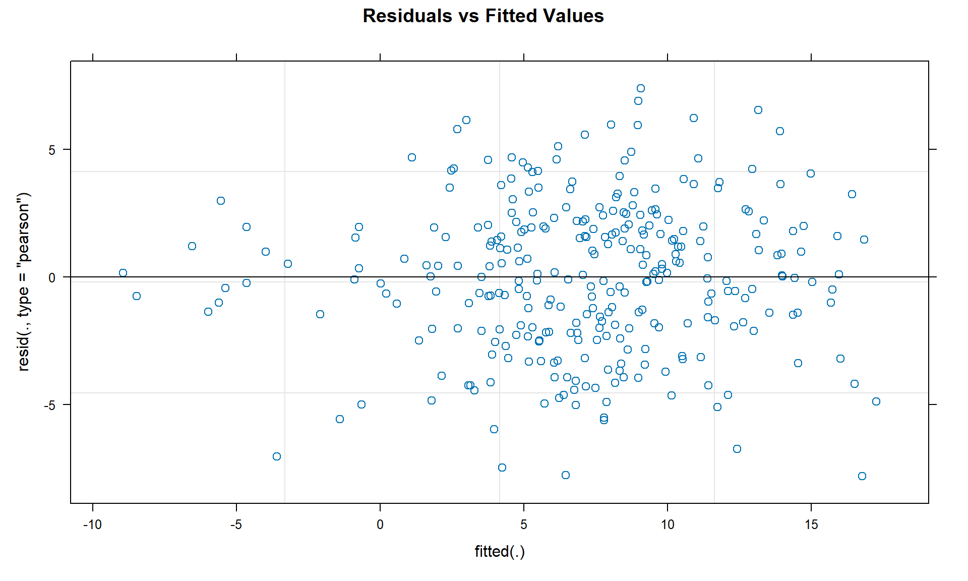
# Q-Q plot of residuals
qqnorm(residuals(model_3), main = "Q-Q Plot of Residuals")
qqline(residuals(model_3))

# Reset plotting parameters
par(mfrow = c(1, 1))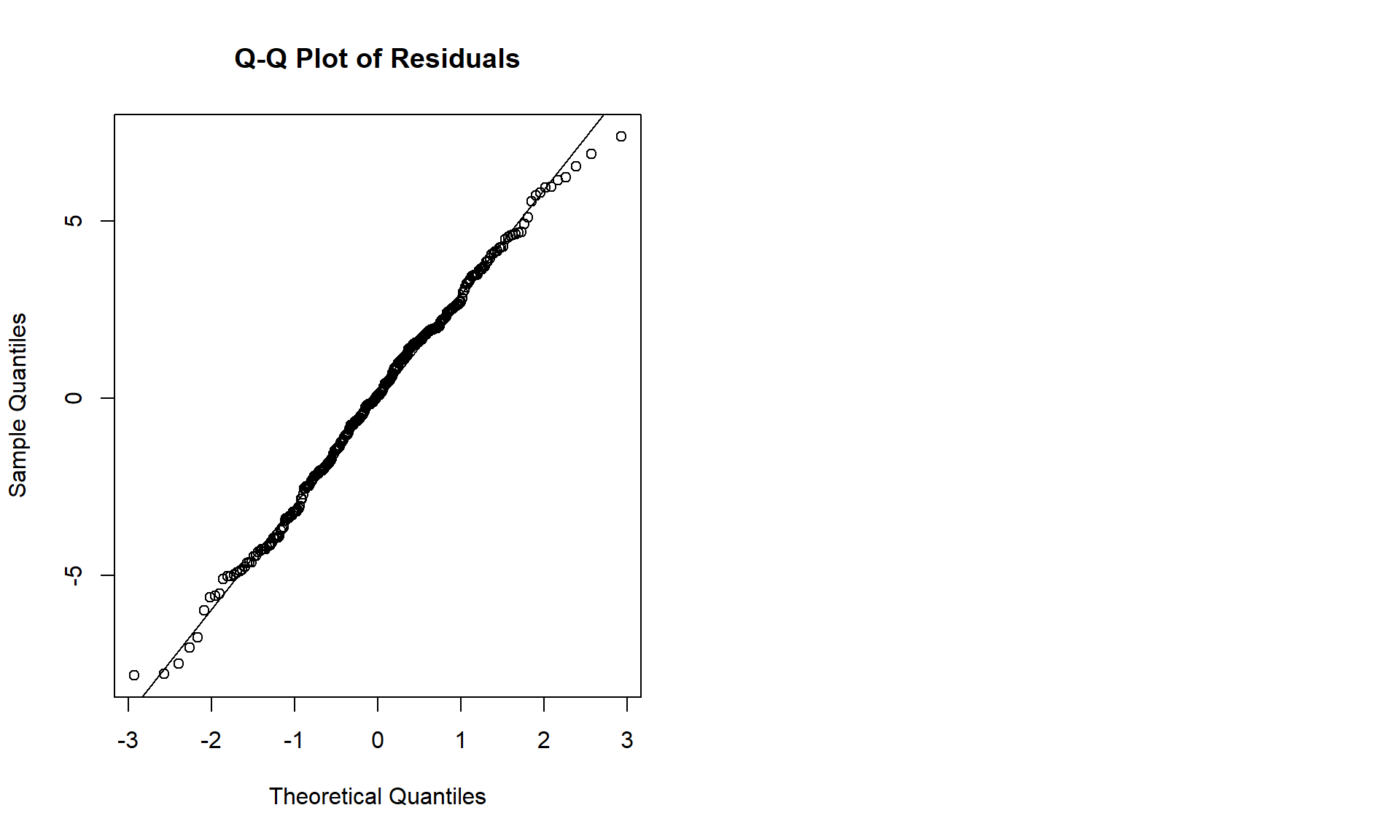
# Additional diagnostic plots
par(mfrow = c(2, 2))

# Scale-Location plot
plot(fitted(model_3), sqrt(abs(residuals(model_3))),
     xlab = "Fitted Values", ylab = "sqrt(|Residuals|)",
     main = "Scale-Location Plot")
abline(h = 0, col = "red", lty = 2)

# Residuals vs Treatment Weeks
plot(full_data$treatment_weeks, residuals(model_3),
     xlab = "Treatment Weeks", ylab = "Residuals",
     main = "Residuals vs Treatment Weeks")
abline(h = 0, col = "red", lty = 2)

# Residuals vs Baseline Depression
plot(full_data$baseline_depression, residuals(model_3),
     xlab = "Baseline Depression", ylab = "Residuals",
     main = "Residuals vs Baseline Depression")
abline(h = 0, col = "red", lty = 2)

# Histogram of residuals
hist(residuals(model_3), breaks = 20,
     main = "Distribution of Residuals", xlab = "Residuals")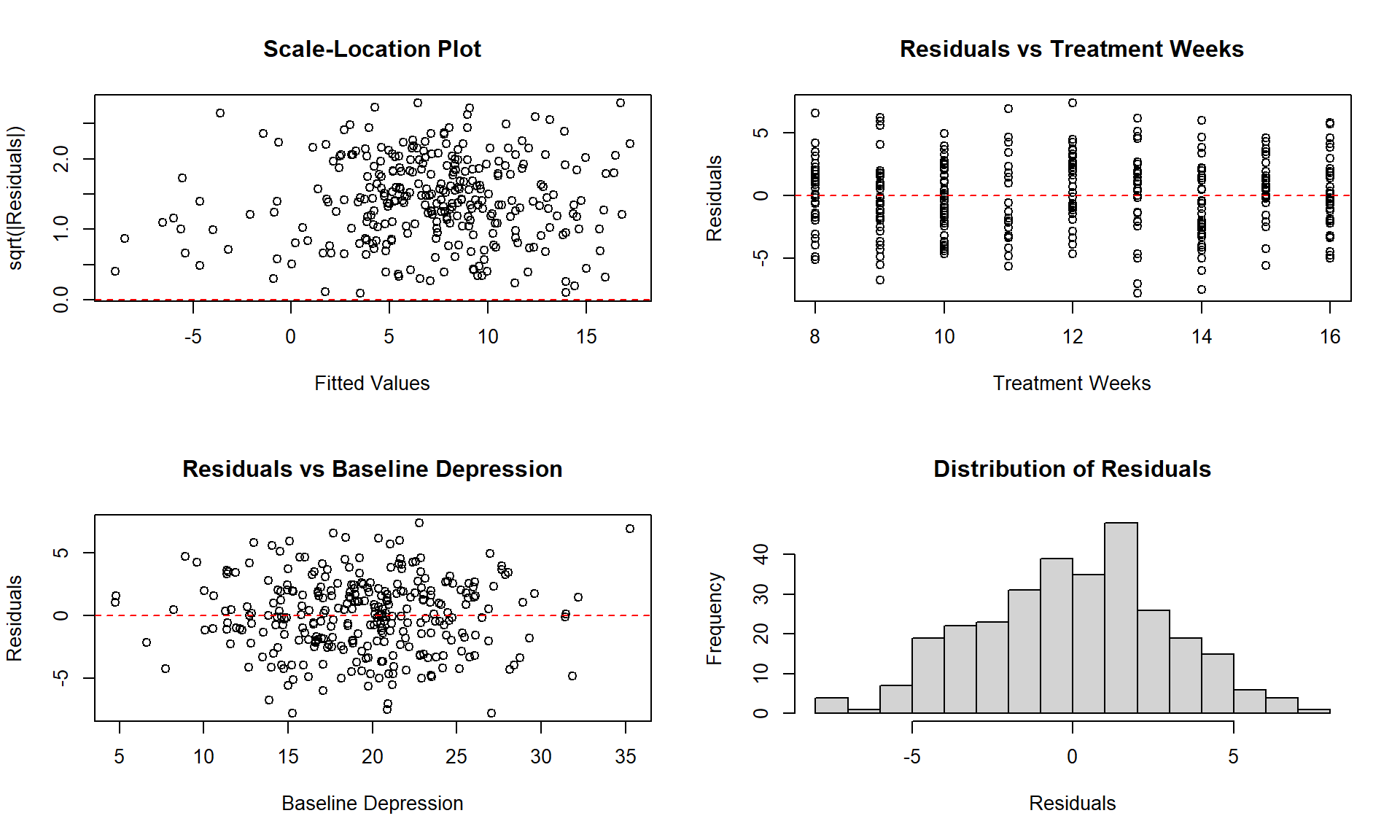
1.19 Visualization of Results
# Marginal effects
marginal_effects <- ggpredict(model_3, terms = c("treatment_weeks", "therapy_approach"))
plot(marginal_effects)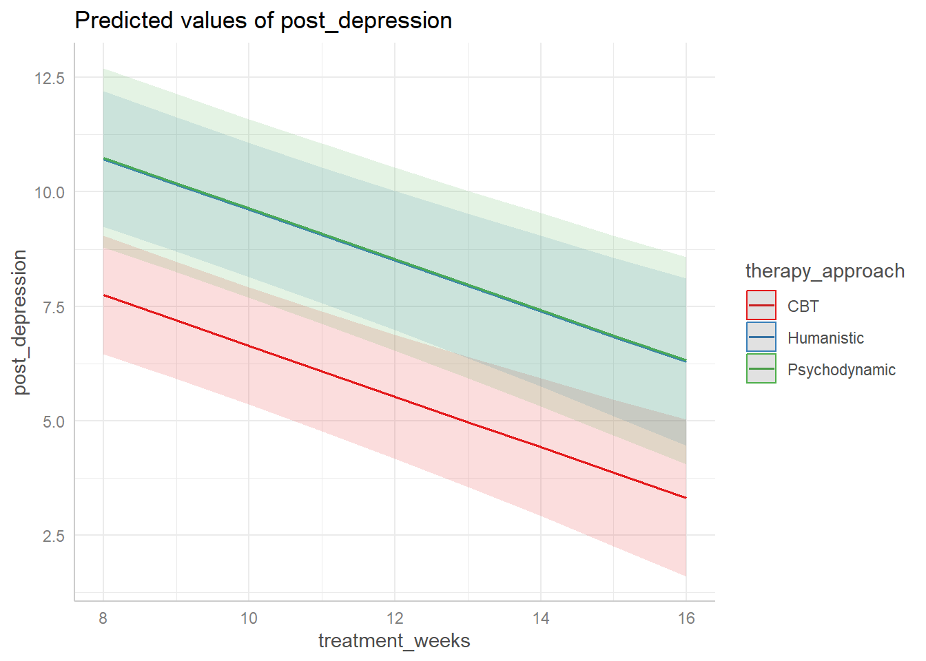
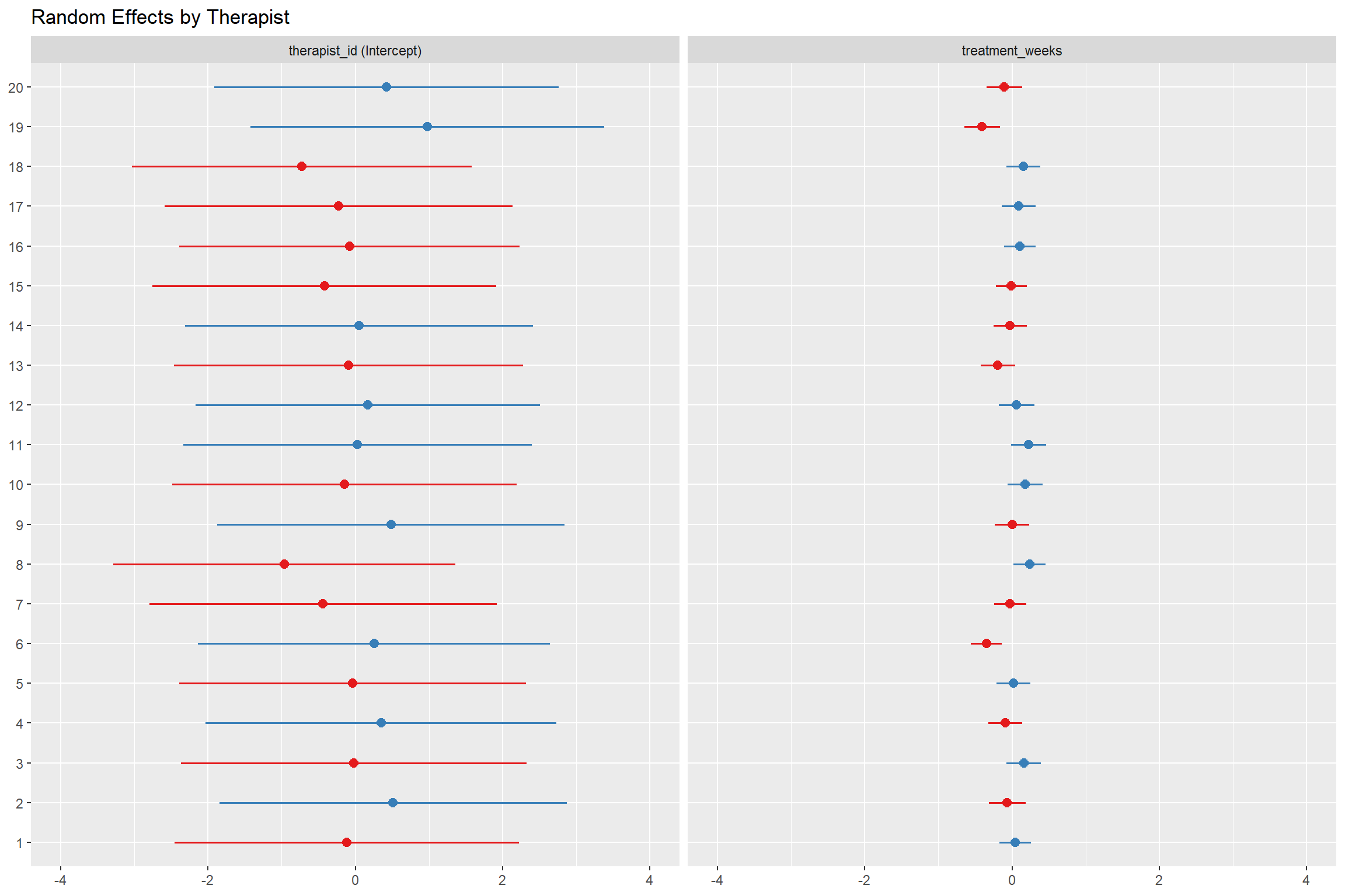
# Random effects by therapist
ranef_plot <- plot_model(model_3, type = "re", sort.est = TRUE)
ranef_plot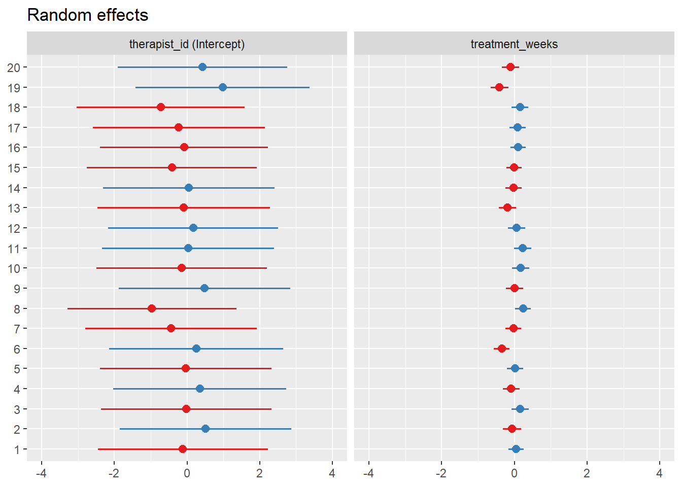
1.20 Interpretation of Results
1.20.1 Fixed Effects Interpretation
##                   (Intercept)           baseline_depression
##                  13.756597259                   0.325484644
##               treatment_weeks                           age
##                  -0.553462298                   0.002394489
##          therapist_experience    therapy_approachHumanistic
##                  -1.513844146                   2.969808670
## therapy_approachPsychodynamic
## 3.000868481## 2.5 % 97.5 %
## .sig01 NA NA
## .sig02 NA NA
## .sig03 NA NA
## .sigma NA NA
## (Intercept) 10.22313316 17.2900614
## baseline_depression 0.25213579 0.3988335
## treatment_weeks -0.72164508 -0.3852795
## age -0.02700512 0.0317941
## therapist_experience -1.97381186 -1.0538764
## therapy_approachHumanistic 1.05071703 4.8889003
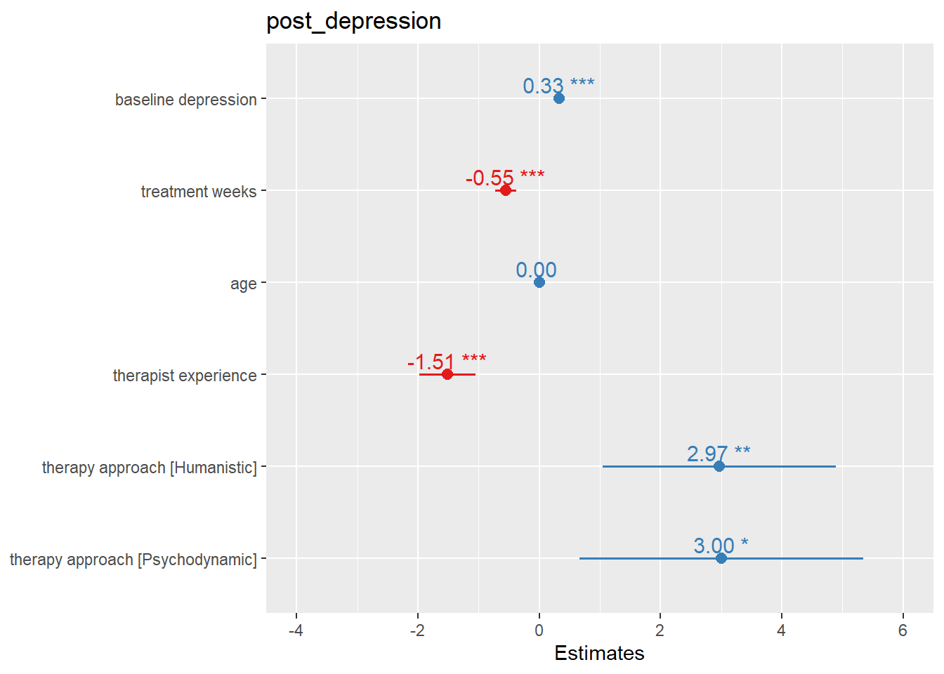
## therapy_approachPsychodynamic 0.66947424 5.3322627The results show:
Baseline Depression: For each 1-point increase in baseline depression, post-treatment depression increases by 0.325 points, holding all other variables constant.
Treatment Weeks: Each additional week of treatment reduces post-treatment depression by 0.553 points on average.
Therapist Experience: Each additional year of therapist experience reduces patient depression by 1.514 points.
Therapy Approach: Compared to humanistic therapy (reference category), CBT reduces depression by an additional 2.97 points, while psychodynamic therapy reduces it by 3.001 points.
1.20.2 Random Effects Interpretation
## $therapist_id
##    (Intercept) treatment_weeks
## 1  -0.11727015    0.0454392926
## 2   0.51332659   -0.0655155602
## 3  -0.02000294    0.1581950727
## 4   0.35144517   -0.0914805088
## 5  -0.03724216    0.0188243242
## 6   0.25488101   -0.3490022816
## 7  -0.43718629   -0.0278116765
## 8  -0.96518264    0.2367664758
## 9   0.48520017   -0.0002873795
## 10 -0.14574576    0.1757882309
## 11  0.02921167    0.2260260429
## 12  0.17090099    0.0612234400
## 13 -0.09295097   -0.1913928895
## 14  0.05135264   -0.0257822873
## 15 -0.41664196   -0.0106300097
## 16 -0.07906114    0.1059293948
## 17 -0.22389885    0.0907071384
## 18 -0.72281381    0.1544625769
## 19  0.97809853   -0.4070093258
## 20  0.42357989   -0.1044500706
##
## with conditional variances for "therapist_id"## Groups Name Std.Dev. Corr
## therapist_id (Intercept) 1.28033
## treatment_weeks 0.21451 -0.616
## Residual 3.04988The random effects show significant variation between therapists in both: - Intercept: Therapists vary in their baseline effectiveness - Treatment Weeks Slope: Therapists vary in how much benefit their patients get from additional treatment weeks
1.21 Effect Sizes and Practical Significance
# Calculate R-squared (proportion of variance explained)
r2_marginal <- performance::r2(model_3)
print(r2_marginal)
## # R2 for Mixed Models
##
## Conditional R2: 0.690
## Marginal R2: 0.540# Cohen's d for therapy approaches
# CBT vs Humanistic
cohen_d_cbt <- abs(fixed_effects[6]) / sigma(model_3)
print(paste("Cohen's d for CBT effect:", round(cohen_d_cbt, 3)))## [1] "Cohen's d for CBT effect: 0.974"# Psychodynamic vs Humanistic
cohen_d_psycho <- abs(fixed_effects[7]) / sigma(model_3)
print(paste("Cohen's d for Psychodynamic effect:", round(cohen_d_psycho, 3)))## [1] "Cohen's d for Psychodynamic effect: 0.984"1.22 Power Analysis and Sample Size Considerations
# Simulate power analysis for different sample sizes
simulate_power <- function(n_therapists, n_patients_per_therapist, effect_size = -0.5) {
  # This is a simplified power simulation
  # In practice, you would use packages like simr or powerlmm

  n_sims <- 100
  significant_results <- 0

  for (i in 1:n_sims) {
    # Simulate data similar to our original simulation
    sim_data <- data.frame(
      therapist_id = as.factor(rep(1:n_therapists, each = n_patients_per_therapist)),
      treatment_weeks = rnorm(n_therapists * n_patients_per_therapist, 12, 3),
      baseline_depression = rnorm(n_therapists * n_patients_per_therapist, 20, 5)
    )

    # Add random effects
    therapist_effects <- rnorm(n_therapists, 0, 2)
    sim_data$therapist_effect <- therapist_effects[as.numeric(sim_data$therapist_id)]

    # Generate outcome
    sim_data$post_depression <- with(sim_data,
      15 + 0.3 * baseline_depression + effect_size * treatment_weeks +
      therapist_effect + rnorm(nrow(sim_data), 0, 3)
    )

    # Fit model
    sim_model <- lmer(post_depression ~ baseline_depression + treatment_weeks +
                      (1 | therapist_id), data = sim_data)

    # Check if treatment effect is significant
    if (summary(sim_model)$coefficients["treatment_weeks", "Pr(>|t|)"] < 0.05) {
      significant_results <- significant_results + 1
    }
  }

  return(significant_results / n_sims)
}

# Calculate power for current sample size
current_power <- simulate_power(n_therapists = 20, n_patients_per_therapist = 15)
print(paste("Estimated power with current sample:", round(current_power, 3)))
## [1] "Estimated power with current sample: 1"1.23 Conclusions and Recommendations
1.23.1 Key Findings:
Multilevel Structure: The ICC indicates that approximately 54.3% of the variance in post-treatment depression is due to differences between therapists, justifying the use of multilevel modeling.
Treatment Effectiveness: Treatment weeks significantly reduce depression scores, with the effect varying across therapists.
Therapist Factors: Both therapist experience and therapy approach significantly influence treatment outcomes.
Model Fit: The full multilevel model explains 54% of the variance in outcomes (marginal R²) and 69% including random effects (conditional R²).
1.23.2 Methodological Considerations:
- Assumption Checking: Always verify model assumptions through diagnostic plots
- Model Selection: Use information criteria (AIC, BIC) and theoretical considerations for model selection
- Effect Sizes: Report both statistical significance and practical significance
- Power Analysis: Consider power analysis for planning future studies
1.23.3 Practical Implications:
- Training: Therapist experience significantly improves outcomes, suggesting value in continued training
- Approach Selection: CBT shows the largest effect size, but individual therapist variation is also important
- Treatment Duration: Longer treatment generally improves outcomes, but with diminishing returns
This analysis demonstrates how multilevel modeling can provide insights into complex behavioral phenomena while accounting for the hierarchical structure of data commonly found in behavioral science research.