Chapter 3 Survival Analysis & Time-to-Event Modeling
3.2 What is Survival Analysis?
Survival analysis, also known as time-to-event analysis, is a statistical method designed to analyze the time until a specific event occurs. Despite its name, survival analysis is not limited to death or medical outcomes - it’s widely used in behavioral science to study any time-dependent event.
3.3 Core Concepts and Terminology
3.3.1 Key Components of Survival Data
- Time Variable: Duration until event occurs (or last observation if censored)
- Event Indicator: Whether the event occurred (1) or was censored (0)
- Covariates: Variables that might influence survival time
3.3.2 Censoring: A Unique Feature
Censoring occurs when we don’t observe the event for some individuals during the study period:
- Right Censoring: Most common - we know the event hasn’t occurred by end of study
- Left Censoring: Event occurred before study began, but we don’t know when
- Interval Censoring: Event occurred within a time interval, but exact time unknown
3.3.3 Why Regular Regression Doesn’t Work
Traditional regression fails with survival data because: 1. Censored observations: Can’t ignore incomplete cases 2. Non-normal distributions: Survival times often follow exponential, Weibull, or log-normal distributions 3. Time-varying effects: Relationships may change over time
3.4 When to Use Survival Analysis
3.4.1 Research Questions Ideal for Survival Analysis:
- Time to Behavioral Change: How long until desired behavior occurs?
- Example: “How long until smoking cessation after intervention?”
- Treatment Duration Effects: What factors influence treatment retention?
- Example: “What predicts longer engagement in therapy?”
- Relapse Prevention: When do negative behaviors return?
- Example: “What factors delay relapse in addiction recovery?”
- Developmental Milestones: When do developmental events occur?
- Example: “What predicts timing of first romantic relationship?”
3.4.2 Real-World Applications in Behavioral Science:
3.4.2.1 Clinical Psychology:
- Question: “How long do patients remain in therapy, and what factors predict dropout?”
- Design: Time from therapy start to dropout (or study end if still enrolled)
- Variables: Therapist experience, patient severity, insurance type
- Insight: Identify early warning signs of dropout for targeted retention efforts
3.4.2.2 Addiction Research:
- Question: “What factors influence time to relapse after substance abuse treatment?”
- Design: Time from treatment completion to first substance use
- Variables: Treatment type, social support, employment status, severity
- Insight: Develop personalized relapse prevention strategies
3.4.2.3 Educational Psychology:
- Question: “How long do students persist in challenging academic programs?”
- Design: Time from program entry to dropout or completion
- Variables: Academic preparation, financial aid, mentorship, motivation
- Insight: Identify students at risk and optimal timing for interventions
3.4.2.4 Organizational Psychology:
- Question: “What predicts employee turnover timing in high-stress jobs?”
- Design: Time from hiring to voluntary resignation
- Variables: Job satisfaction, supervisor support, workload, compensation
- Insight: Optimize retention strategies and identify critical time periods
3.5 Advantages of Survival Analysis
3.7 Types of Survival Analysis
3.7.1 1. Kaplan-Meier (Non-parametric)
- Purpose: Estimate survival curves without assumptions about distribution
- Use when: Descriptive analysis or comparing groups
- Example: “What percentage of patients remain in therapy at 6 months?”
3.7.2 2. Cox Proportional Hazards (Semi-parametric)
- Purpose: Test covariate effects without specifying baseline hazard shape
- Use when: Primary interest is in risk factors, not absolute survival times
- Example: “How does therapist experience affect therapy retention?”
3.8 Key Survival Analysis Concepts
3.8.1 Hazard Ratio (HR)
- Interpretation: Relative risk of event at any given time
- HR = 1: No effect
- HR > 1: Increased risk (shorter survival)
- HR < 1: Decreased risk (longer survival)
3.9 Research Questions Addressed by Survival Analysis
3.9.1 1. Group Comparisons
- Question: “Do patients in CBT vs. medication survive longer without relapse?”
- Analysis: Kaplan-Meier curves with log-rank test
3.9.2 2. Risk Factor Identification
- Question: “What baseline characteristics predict faster therapy dropout?”
- Analysis: Cox proportional hazards model
3.10 How to Report Survival Analysis Results in APA Format
3.10.1 Kaplan-Meier Results:
“Kaplan-Meier analysis revealed that median time to therapy dropout was 12.3 weeks (95% CI [10.1, 14.8]). The 6-month retention rate was 68% (95% CI [62%, 74%]).”
3.10.2 Cox Model Results:
“Cox proportional hazards regression indicated that higher baseline severity significantly increased dropout risk (HR = 1.15, 95% CI [1.08, 1.23], p < .001), while greater social support was protective (HR = 0.82, 95% CI [0.71, 0.95], p = .008).”
3.10.3 Hazard Ratio Interpretation:
“Patients with high baseline severity had a 15% higher risk of dropout at any given time compared to those with low severity.”
3.10.4 Model Fit:
“The model demonstrated good discriminative ability (C-index = .72) and overall significance (likelihood ratio test: χ² = 45.3, df = 6, p < .001).”
Understanding these concepts enables researchers to appropriately apply survival analysis to answer important questions about timing and duration in behavioral science research.
3.11 Mathematical Foundation
3.11.1 Survival Function
The survival function \(S(t)\) represents the probability that an individual survives beyond time \(t\): \[S(t) = P(T > t) = 1 - F(t)\]
3.12 Required Packages
# Set CRAN mirror
options(repos = c(CRAN = "https://cran.rstudio.com/"))

# Install packages if not already installed
if (!require("survival")) install.packages("survival")
if (!require("survminer")) install.packages("survminer")
if (!require("report")) install.packages("report")
if (!require("ggplot2")) install.packages("ggplot2")
if (!require("dplyr")) install.packages("dplyr")
if (!require("tidyr")) install.packages("tidyr")
if (!require("KMsurv")) install.packages("KMsurv")
if (!require("flexsurv")) install.packages("flexsurv")
if (!require("ggfortify")) install.packages("ggfortify")

library(survival)
library(survminer)
library(report)
library(ggplot2)
library(dplyr)
library(tidyr)
library(KMsurv)
library(flexsurv)
library(ggfortify)
3.13 Data Simulation: Addiction Treatment Study
We’ll simulate a dataset examining time to relapse in an addiction treatment program, considering various patient characteristics and treatment modalities.
set.seed(789)
n <- 400

# Generate baseline characteristics
addiction_data <- data.frame(
  patient_id = 1:n,
  age = round(rnorm(n, mean = 35, sd = 10)),
  gender = sample(c("Male", "Female"), n, replace = TRUE, prob = c(0.6, 0.4)),
  treatment_type = sample(c("Inpatient", "Outpatient", "Intensive_Outpatient"),
                         n, replace = TRUE, prob = c(0.3, 0.4, 0.3)),
  severity_score = round(rnorm(n, mean = 15, sd = 5)), # Addiction severity (1-30)
  social_support = round(rnorm(n, mean = 7, sd = 2)), # Social support scale (1-10)
  previous_treatments = rpois(n, lambda = 1.5), # Number of previous treatments
  motivation_score = round(rnorm(n, mean = 8, sd = 2)) # Motivation scale (1-10)
)

# Ensure realistic ranges
addiction_data$age[addiction_data$age < 18] <- 18
addiction_data$age[addiction_data$age > 70] <- 70
addiction_data$severity_score[addiction_data$severity_score < 1] <- 1
addiction_data$severity_score[addiction_data$severity_score > 30] <- 30
addiction_data$social_support[addiction_data$social_support < 1] <- 1
addiction_data$social_support[addiction_data$social_support > 10] <- 10
addiction_data$motivation_score[addiction_data$motivation_score < 1] <- 1
addiction_data$motivation_score[addiction_data$motivation_score > 10] <- 10

# Create dummy variables for Cox regression
addiction_data$gender_male <- ifelse(addiction_data$gender == "Male", 1, 0)
addiction_data$treatment_inpatient <- ifelse(addiction_data$treatment_type == "Inpatient", 1, 0)
addiction_data$treatment_intensive <- ifelse(addiction_data$treatment_type == "Intensive_Outpatient", 1, 0)

# Generate survival times using Weibull distribution with covariates
# Linear predictor
lp <- with(addiction_data,
  -0.02 * age +                    # Older age slightly protective
  0.3 * gender_male +              # Males higher risk
  -0.5 * treatment_inpatient +     # Inpatient treatment protective
  -0.3 * treatment_intensive +     # Intensive outpatient protective
  0.08 * severity_score +          # Higher severity = higher risk
  -0.15 * social_support +         # More support = lower risk
  0.2 * previous_treatments +      # More previous treatments = higher risk
  -0.1 * motivation_score          # Higher motivation = lower risk
)

# Generate survival times (Weibull distribution)
shape_param <- 1.5
scale_param <- exp(-lp)
survival_time <- rweibull(n, shape = shape_param, scale = scale_param)

# Convert to days and add some realism (max 365 days follow-up)
addiction_data$time_to_event <- round(survival_time * 100)
addiction_data$time_to_event[addiction_data$time_to_event > 365] <- 365

# Generate censoring (lost to follow-up)
# Higher dropout for outpatient, lower motivation, etc.
dropout_prob <- with(addiction_data,
  0.15 +
  0.1 * (treatment_type == "Outpatient") +
  0.05 * (motivation_score <= 5) +
  0.03 * (social_support <= 4)
)

addiction_data$censored <- rbinom(n, 1, dropout_prob)

# For censored observations, use random censoring time
censoring_times <- runif(sum(addiction_data$censored),
                        min = 30, max = 365)
addiction_data$time_to_event[addiction_data$censored == 1] <-
  round(censoring_times)

# Create event indicator (1 = relapse, 0 = censored)
addiction_data$event <- 1 - addiction_data$censored

# Convert categorical variables to factors
addiction_data$gender <- as.factor(addiction_data$gender)
addiction_data$treatment_type <- as.factor(addiction_data$treatment_type)

# Display first few rows
head(addiction_data, 10)
## patient_id age gender treatment_type severity_score social_support
## 1 1 40 Female Intensive_Outpatient 27 8
## 2 2 18 Male Inpatient 9 4
## 3 3 35 Female Outpatient 13 6
## 4 4 37 Male Intensive_Outpatient 17 2
## 5 5 31 Male Outpatient 8 6
## 6 6 30 Male Outpatient 17 7
## 7 7 28 Male Intensive_Outpatient 4 6
## 8 8 33 Male Inpatient 11 7
## 9 9 25 Female Inpatient 9 3
## 10 10 42 Male Intensive_Outpatient 22 5
## previous_treatments motivation_score gender_male treatment_inpatient
## 1 1 10 0 0
## 2 0 9 1 1
## 3 2 10 0 0
## 4 2 8 1 0
## 5 1 6 1 0
## 6 3 9 1 0
## 7 2 10 1 0
## 8 2 9 1 1
## 9 3 8 0 1
## 10 2 10 1 0
## treatment_intensive time_to_event censored event
## 1 1 287 0 1
## 2 0 228 0 1
## 3 0 365 0 1
## 4 1 30 0 1
## 5 0 88 0 1
## 6 0 175 0 1
## 7 1 361 0 1
## 8 0 365 0 1
## 9 0 88 0 1
## 10 1 151 0 1# Summary of key variables
summary(addiction_data[, c("time_to_event", "event", "age", "severity_score",
"social_support", "motivation_score")])## time_to_event event age severity_score
## Min. : 1.0 Min. :0.0000 Min. :18.00 Min. : 1.00
## 1st Qu.:104.8 1st Qu.:1.0000 1st Qu.:28.00 1st Qu.:11.00
## Median :218.0 Median :1.0000 Median :35.00 Median :15.00
## Mean :216.6 Mean :0.8025 Mean :35.04 Mean :14.91
## 3rd Qu.:361.5 3rd Qu.:1.0000 3rd Qu.:42.00 3rd Qu.:18.00
## Max. :365.0 Max. :1.0000 Max. :66.00 Max. :28.00
## social_support motivation_score
## Min. : 1.000 Min. : 2.000
## 1st Qu.: 6.000 1st Qu.: 7.000
## Median : 7.000 Median : 8.000
## Mean : 6.848 Mean : 7.718
## 3rd Qu.: 8.000 3rd Qu.: 9.000
## Max. :10.000 Max. :10.000##
## Inpatient Intensive_Outpatient Outpatient
## 0 15 18 46
## 1 102 102 1173.14 Exploratory Data Analysis
# Event rates by treatment type
event_summary <- addiction_data %>%
  group_by(treatment_type) %>%
  summarise(
    n = n(),
    events = sum(event),
    event_rate = mean(event),
    median_time = median(time_to_event),
    .groups = 'drop'
  )
print(event_summary)
## # A tibble: 3 × 5
## treatment_type n events event_rate median_time
## <fct> <int> <dbl> <dbl> <dbl>
## 1 Inpatient 117 102 0.872 256
## 2 Intensive_Outpatient 120 102 0.85 229
## 3 Outpatient 163 117 0.718 172# Distribution of survival times
ggplot(addiction_data, aes(x = time_to_event, fill = factor(event))) +
geom_histogram(bins = 30, alpha = 0.7, position = "identity") +
facet_wrap(~ treatment_type) +
labs(title = "Distribution of Time to Event by Treatment Type",
x = "Time to Event (days)",
y = "Frequency",
fill = "Event") +
scale_fill_discrete(labels = c("Censored", "Relapse")) +
theme_minimal()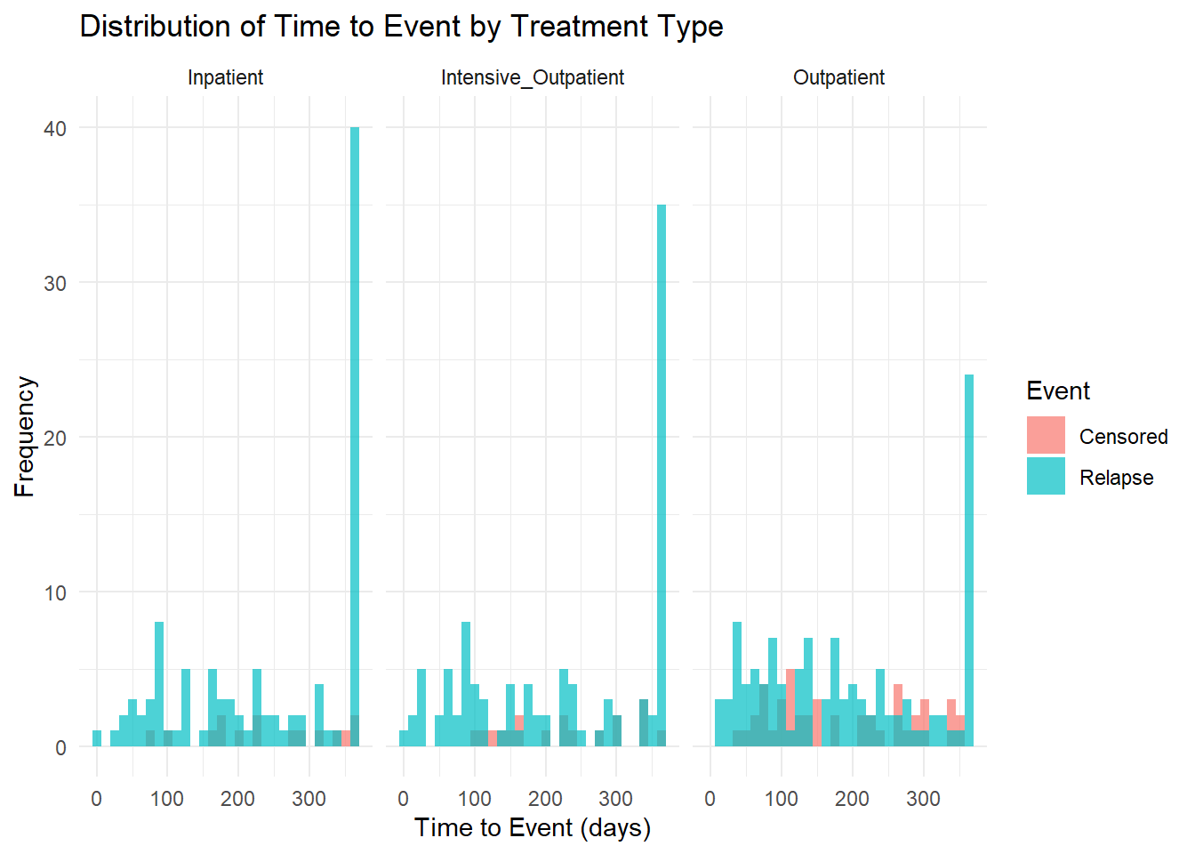
# Boxplot of key variables by event status
addiction_data %>%
  select(event, age, severity_score, social_support, motivation_score) %>%
  pivot_longer(cols = -event, names_to = "variable", values_to = "value") %>%
  ggplot(aes(x = factor(event), y = value, fill = factor(event))) +
  geom_boxplot(alpha = 0.7) +
  facet_wrap(~ variable, scales = "free_y") +
  labs(title = "Distribution of Variables by Event Status",
       x = "Event Status",
       y = "Value",
       fill = "Event") +
  scale_x_discrete(labels = c("Censored", "Relapse")) +
  scale_fill_discrete(labels = c("Censored", "Relapse")) +
  theme_minimal()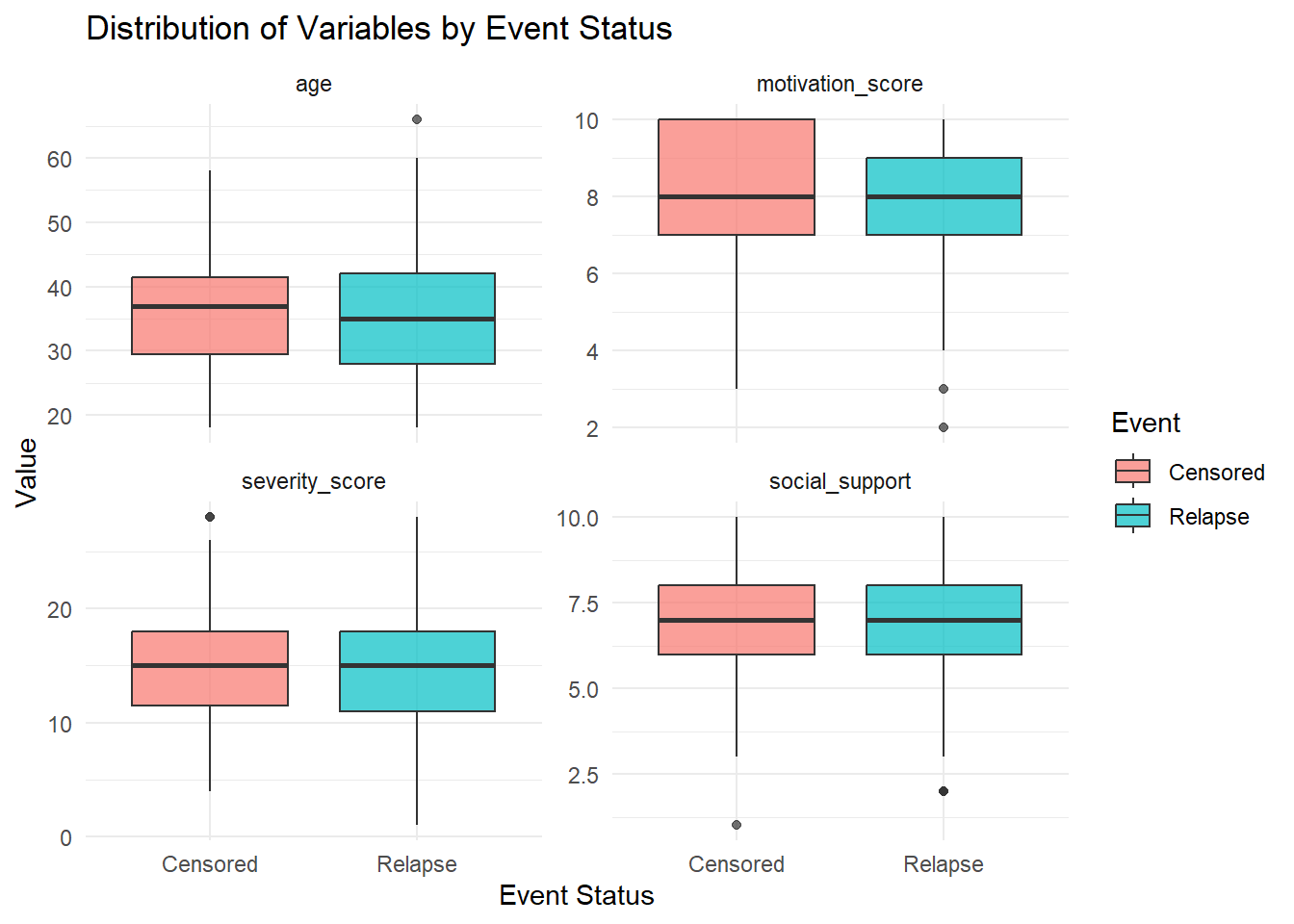
3.15 Kaplan-Meier Survival Analysis
# Create survival object
surv_object <- Surv(time = addiction_data$time_to_event,
                   event = addiction_data$event)

# Overall survival curve
km_fit <- survfit(surv_object ~ 1, data = addiction_data)
summary(km_fit)
## Call: survfit(formula = surv_object ~ 1, data = addiction_data)
##
## time n.risk n.event survival std.err lower 95% CI upper 95% CI
## 1 400 1 0.99750 0.00250 0.992618 1.0000
## 5 399 1 0.99500 0.00353 0.988112 1.0000
## 8 398 1 0.99250 0.00431 0.984081 1.0000
## 9 397 2 0.98750 0.00556 0.976672 0.9984
## 14 395 1 0.98500 0.00608 0.973160 0.9970
## 16 394 1 0.98250 0.00656 0.969734 0.9954
## 19 393 1 0.98000 0.00700 0.966376 0.9938
## 22 392 2 0.97500 0.00781 0.959819 0.9904
## 24 390 2 0.97000 0.00853 0.953426 0.9869
## 25 388 1 0.96750 0.00887 0.950278 0.9850
## 26 387 1 0.96500 0.00919 0.947157 0.9832
## 30 386 1 0.96250 0.00950 0.944061 0.9813
## 31 385 1 0.96000 0.00980 0.940987 0.9794
## 33 384 3 0.95250 0.01064 0.931882 0.9736
## 34 381 3 0.94500 0.01140 0.922920 0.9676
## 35 378 2 0.94000 0.01187 0.917012 0.9636
## 39 375 1 0.93749 0.01210 0.914067 0.9615
## 43 374 1 0.93499 0.01233 0.911132 0.9595
## 44 373 2 0.92997 0.01276 0.905293 0.9553
## 45 371 1 0.92747 0.01297 0.902388 0.9532
## 46 370 1 0.92496 0.01318 0.899492 0.9511
## 50 369 1 0.92245 0.01338 0.896604 0.9490
## 52 367 2 0.91743 0.01377 0.890834 0.9448
## 53 365 2 0.91240 0.01414 0.885094 0.9405
## 57 363 2 0.90737 0.01451 0.879381 0.9363
## 60 361 1 0.90486 0.01468 0.876535 0.9341
## 63 358 2 0.89980 0.01503 0.870824 0.9297
## 64 356 1 0.89728 0.01520 0.867978 0.9276
## 65 355 1 0.89475 0.01536 0.865137 0.9254
## 66 354 1 0.89222 0.01553 0.862302 0.9232
## 67 353 1 0.88969 0.01569 0.859472 0.9210
## 68 352 1 0.88717 0.01584 0.856648 0.9188
## 69 351 2 0.88211 0.01615 0.851013 0.9143
## 70 349 1 0.87958 0.01630 0.848203 0.9121
## 72 348 1 0.87706 0.01645 0.845398 0.9099
## 77 344 1 0.87451 0.01660 0.842569 0.9077
## 79 342 3 0.86684 0.01703 0.834083 0.9009
## 80 339 1 0.86428 0.01718 0.831263 0.8986
## 81 337 2 0.85915 0.01745 0.825616 0.8940
## 82 335 2 0.85402 0.01772 0.819985 0.8895
## 83 333 1 0.85146 0.01785 0.817175 0.8872
## 84 331 5 0.83859 0.01849 0.803133 0.8756
## 85 326 2 0.83345 0.01873 0.797541 0.8710
## 86 324 3 0.82573 0.01908 0.789176 0.8640
## 87 321 2 0.82059 0.01930 0.783616 0.8593
## 88 319 3 0.81287 0.01963 0.775297 0.8523
## 90 316 1 0.81030 0.01973 0.772530 0.8499
## 92 315 2 0.80515 0.01994 0.767004 0.8452
## 93 313 2 0.80001 0.02014 0.761489 0.8405
## 95 311 2 0.79486 0.02034 0.755984 0.8357
## 96 307 2 0.78968 0.02053 0.750450 0.8310
## 99 304 1 0.78709 0.02063 0.747676 0.8286
## 104 302 2 0.78187 0.02082 0.742117 0.8238
## 105 300 1 0.77927 0.02091 0.739341 0.8214
## 106 299 1 0.77666 0.02100 0.736567 0.8189
## 112 294 1 0.77402 0.02110 0.733755 0.8165
## 115 292 2 0.76872 0.02128 0.728115 0.8116
## 117 290 1 0.76607 0.02137 0.725299 0.8091
## 118 289 1 0.76342 0.02146 0.722486 0.8067
## 120 286 1 0.76075 0.02155 0.719653 0.8042
## 121 284 1 0.75807 0.02164 0.716812 0.8017
## 123 282 2 0.75269 0.02182 0.711114 0.7967
## 124 280 1 0.75000 0.02191 0.708269 0.7942
## 125 278 2 0.74461 0.02208 0.702564 0.7892
## 129 276 1 0.74191 0.02217 0.699714 0.7867
## 130 275 2 0.73652 0.02233 0.694023 0.7816
## 134 272 1 0.73381 0.02241 0.691170 0.7791
## 135 270 1 0.73109 0.02249 0.688307 0.7765
## 138 268 2 0.72563 0.02265 0.682565 0.7714
## 139 266 1 0.72291 0.02273 0.679697 0.7689
## 141 265 1 0.72018 0.02281 0.676831 0.7663
## 142 264 1 0.71745 0.02289 0.673968 0.7637
## 144 263 1 0.71472 0.02296 0.671108 0.7612
## 145 262 1 0.71199 0.02303 0.668249 0.7586
## 146 261 1 0.70927 0.02311 0.665393 0.7560
## 148 258 1 0.70652 0.02318 0.662514 0.7534
## 151 256 1 0.70376 0.02325 0.659625 0.7508
## 154 254 1 0.70099 0.02333 0.656726 0.7482
## 157 253 2 0.69545 0.02347 0.650935 0.7430
## 159 250 3 0.68710 0.02368 0.642226 0.7351
## 160 247 1 0.68432 0.02374 0.639328 0.7325
## 162 246 1 0.68154 0.02381 0.636432 0.7298
## 165 243 1 0.67873 0.02388 0.633512 0.7272
## 168 242 1 0.67593 0.02394 0.630594 0.7245
## 170 241 1 0.67312 0.02401 0.627678 0.7219
## 171 240 2 0.66751 0.02413 0.621852 0.7165
## 172 237 2 0.66188 0.02425 0.616009 0.7112
## 175 235 1 0.65906 0.02431 0.613090 0.7085
## 176 232 2 0.65338 0.02443 0.607204 0.7031
## 177 230 1 0.65054 0.02449 0.604265 0.7004
## 178 229 3 0.64202 0.02466 0.595458 0.6922
## 179 226 1 0.63918 0.02472 0.592527 0.6895
## 180 225 1 0.63634 0.02477 0.589598 0.6868
## 186 223 1 0.63348 0.02482 0.586657 0.6840
## 190 222 1 0.63063 0.02487 0.583718 0.6813
## 191 221 1 0.62778 0.02492 0.580780 0.6786
## 193 220 3 0.61922 0.02507 0.571981 0.6704
## 194 217 2 0.61351 0.02516 0.566126 0.6649
## 199 214 4 0.60204 0.02533 0.554379 0.6538
## 202 210 1 0.59917 0.02538 0.551447 0.6510
## 203 209 1 0.59631 0.02542 0.548518 0.6483
## 205 207 1 0.59343 0.02546 0.545574 0.6455
## 207 206 1 0.59055 0.02549 0.542633 0.6427
## 210 205 1 0.58767 0.02553 0.539694 0.6399
## 213 204 1 0.58478 0.02557 0.536757 0.6371
## 214 203 1 0.58190 0.02561 0.533822 0.6343
## 218 201 1 0.57901 0.02564 0.530873 0.6315
## 221 199 1 0.57610 0.02568 0.527910 0.6287
## 222 197 2 0.57025 0.02575 0.521956 0.6230
## 224 194 2 0.56437 0.02581 0.515977 0.6173
## 225 192 1 0.56143 0.02585 0.512991 0.6144
## 227 190 1 0.55848 0.02588 0.509990 0.6116
## 228 189 1 0.55552 0.02591 0.506991 0.6087
## 230 188 1 0.55257 0.02594 0.503994 0.6058
## 231 186 2 0.54663 0.02600 0.497970 0.6000
## 232 183 1 0.54364 0.02603 0.494944 0.5971
## 233 181 2 0.53763 0.02609 0.488861 0.5913
## 235 179 2 0.53162 0.02614 0.482787 0.5854
## 237 177 1 0.52862 0.02616 0.479753 0.5825
## 238 176 1 0.52562 0.02619 0.476722 0.5795
## 239 175 3 0.51661 0.02625 0.467641 0.5707
## 240 172 2 0.51060 0.02628 0.461598 0.5648
## 245 168 1 0.50756 0.02630 0.458540 0.5618
## 254 167 1 0.50452 0.02632 0.455484 0.5588
## 256 166 3 0.49540 0.02637 0.446332 0.5499
## 259 163 1 0.49236 0.02638 0.443285 0.5469
## 264 161 1 0.48931 0.02639 0.440220 0.5439
## 269 158 1 0.48621 0.02641 0.437115 0.5408
## 272 155 2 0.47994 0.02643 0.430823 0.5346
## 273 153 1 0.47680 0.02645 0.427681 0.5316
## 281 150 3 0.46726 0.02649 0.418132 0.5222
## 284 146 1 0.46406 0.02650 0.414930 0.5190
## 287 143 1 0.46082 0.02651 0.411682 0.5158
## 288 142 1 0.45757 0.02652 0.408436 0.5126
## 292 141 1 0.45433 0.02653 0.405194 0.5094
## 294 140 2 0.44784 0.02655 0.398717 0.5030
## 303 136 1 0.44454 0.02655 0.395431 0.4998
## 304 135 1 0.44125 0.02656 0.392147 0.4965
## 306 132 1 0.43791 0.02657 0.388812 0.4932
## 311 130 1 0.43454 0.02658 0.385451 0.4899
## 315 129 1 0.43117 0.02658 0.382093 0.4866
## 316 128 1 0.42780 0.02659 0.378739 0.4832
## 317 127 1 0.42443 0.02659 0.375388 0.4799
## 319 125 1 0.42104 0.02659 0.372011 0.4765
## 320 124 1 0.41764 0.02660 0.368637 0.4732
## 321 123 1 0.41425 0.02660 0.365267 0.4698
## 331 122 1 0.41085 0.02659 0.361900 0.4664
## 332 121 1 0.40746 0.02659 0.358537 0.4631
## 336 120 1 0.40406 0.02658 0.355177 0.4597
## 337 118 2 0.39721 0.02657 0.348404 0.4529
## 340 115 1 0.39376 0.02656 0.344990 0.4494
## 344 109 1 0.39015 0.02656 0.341406 0.4458
## 350 105 1 0.38643 0.02657 0.337711 0.4422
## 354 104 1 0.38271 0.02657 0.334021 0.4385
## 356 103 1 0.37900 0.02657 0.330336 0.4348
## 361 101 1 0.37525 0.02657 0.326616 0.4311
## 363 100 1 0.37149 0.02657 0.322900 0.4274
## 365 98 97 0.00379 0.00378 0.000537 0.0268# Plot overall survival curve
ggsurvplot(km_fit,
data = addiction_data,
title = "Overall Survival Curve: Time to Relapse",
xlab = "Time (days)",
ylab = "Probability of Remaining Sober",
conf.int = TRUE,
risk.table = TRUE,
ggtheme = theme_minimal())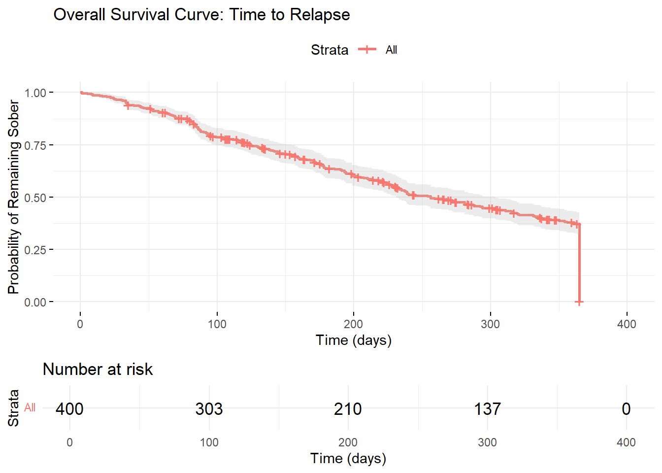
3.16 Survival Analysis by Treatment Type
# Kaplan-Meier by treatment type
km_treatment <- survfit(surv_object ~ treatment_type, data = addiction_data)
summary(km_treatment)
## Call: survfit(formula = surv_object ~ treatment_type, data = addiction_data)
##
## treatment_type=Inpatient
## time n.risk n.event survival std.err lower 95% CI upper 95% CI
## 5 117 1 0.9915 0.00851 0.97491 1.0000
## 25 116 1 0.9829 0.01198 0.95970 1.0000
## 33 115 1 0.9744 0.01461 0.94614 1.0000
## 34 114 1 0.9658 0.01680 0.93344 0.9993
## 44 113 1 0.9573 0.01870 0.92131 0.9946
## 46 112 1 0.9487 0.02039 0.90958 0.9895
## 50 111 1 0.9402 0.02193 0.89816 0.9841
## 57 110 1 0.9316 0.02333 0.88700 0.9785
## 67 109 1 0.9231 0.02464 0.87603 0.9726
## 72 108 1 0.9145 0.02585 0.86525 0.9666
## 79 106 1 0.9059 0.02700 0.85449 0.9604
## 81 105 1 0.8973 0.02809 0.84387 0.9541
## 82 104 1 0.8886 0.02912 0.83337 0.9476
## 84 103 3 0.8628 0.03187 0.80250 0.9276
## 85 100 1 0.8541 0.03270 0.79239 0.9207
## 87 99 1 0.8455 0.03349 0.78235 0.9138
## 88 98 2 0.8283 0.03496 0.76249 0.8997
## 95 96 1 0.8196 0.03564 0.75266 0.8925
## 117 94 1 0.8109 0.03631 0.74276 0.8853
## 120 93 1 0.8022 0.03696 0.73293 0.8780
## 121 92 1 0.7935 0.03757 0.72315 0.8706
## 123 91 1 0.7847 0.03815 0.71342 0.8632
## 124 90 1 0.7760 0.03871 0.70374 0.8557
## 125 89 1 0.7673 0.03925 0.69411 0.8482
## 148 88 1 0.7586 0.03976 0.68453 0.8407
## 157 87 1 0.7499 0.04025 0.67499 0.8331
## 159 85 2 0.7322 0.04119 0.65579 0.8176
## 160 83 1 0.7234 0.04163 0.64625 0.8098
## 165 82 1 0.7146 0.04204 0.63675 0.8019
## 171 81 1 0.7058 0.04244 0.62729 0.7940
## 178 79 1 0.6968 0.04283 0.61774 0.7860
## 180 78 1 0.6879 0.04321 0.60822 0.7780
## 191 76 1 0.6788 0.04357 0.59859 0.7699
## 193 75 1 0.6698 0.04392 0.58901 0.7617
## 194 74 1 0.6607 0.04425 0.57946 0.7534
## 199 72 1 0.6516 0.04458 0.56979 0.7451
## 203 71 1 0.6424 0.04489 0.56017 0.7367
## 213 70 1 0.6332 0.04517 0.55058 0.7282
## 221 69 1 0.6240 0.04544 0.54103 0.7198
## 222 68 1 0.6149 0.04569 0.53152 0.7113
## 227 66 1 0.6055 0.04594 0.52188 0.7026
## 228 65 1 0.5962 0.04617 0.51227 0.6939
## 231 64 1 0.5869 0.04638 0.50270 0.6852
## 233 62 1 0.5774 0.04658 0.49299 0.6764
## 240 61 1 0.5680 0.04677 0.48332 0.6675
## 254 60 1 0.5585 0.04694 0.47369 0.6585
## 256 59 1 0.5490 0.04709 0.46409 0.6495
## 269 58 1 0.5396 0.04722 0.45453 0.6405
## 281 56 2 0.5203 0.04746 0.43513 0.6222
## 288 53 1 0.5105 0.04757 0.42528 0.6128
## 294 52 1 0.5007 0.04766 0.41546 0.6034
## 315 51 1 0.4909 0.04772 0.40569 0.5939
## 316 50 1 0.4810 0.04777 0.39596 0.5844
## 319 48 1 0.4710 0.04781 0.38604 0.5747
## 320 47 1 0.4610 0.04783 0.37616 0.5650
## 321 46 1 0.4510 0.04783 0.36633 0.5552
## 336 45 1 0.4410 0.04781 0.35654 0.5453
## 365 41 40 0.0108 0.01069 0.00153 0.0754
##
## treatment_type=Intensive_Outpatient
## time n.risk n.event survival std.err lower 95% CI upper 95% CI
## 1 120 1 0.992 0.0083 0.976 1.000
## 9 119 1 0.983 0.0117 0.961 1.000
## 16 118 1 0.975 0.0143 0.947 1.000
## 22 117 1 0.967 0.0164 0.935 0.999
## 24 116 2 0.950 0.0199 0.912 0.990
## 30 114 1 0.942 0.0214 0.901 0.985
## 31 113 1 0.933 0.0228 0.890 0.979
## 52 112 2 0.917 0.0252 0.869 0.967
## 64 110 1 0.908 0.0263 0.858 0.961
## 65 109 1 0.900 0.0274 0.848 0.955
## 68 108 1 0.892 0.0284 0.838 0.949
## 69 107 2 0.875 0.0302 0.818 0.936
## 80 105 1 0.867 0.0310 0.808 0.930
## 81 104 1 0.858 0.0318 0.798 0.923
## 84 103 2 0.842 0.0333 0.779 0.910
## 85 101 1 0.833 0.0340 0.769 0.903
## 86 100 2 0.817 0.0353 0.750 0.889
## 87 98 1 0.808 0.0359 0.741 0.882
## 90 97 1 0.800 0.0365 0.732 0.875
## 93 96 1 0.792 0.0371 0.722 0.868
## 95 95 1 0.783 0.0376 0.713 0.861
## 96 94 1 0.775 0.0381 0.704 0.853
## 104 92 1 0.767 0.0386 0.694 0.846
## 106 91 1 0.758 0.0391 0.685 0.839
## 112 89 1 0.750 0.0396 0.676 0.831
## 115 88 1 0.741 0.0400 0.667 0.824
## 118 87 1 0.733 0.0405 0.657 0.816
## 142 84 1 0.724 0.0409 0.648 0.809
## 145 83 1 0.715 0.0414 0.639 0.801
## 146 82 1 0.706 0.0418 0.629 0.793
## 151 81 1 0.698 0.0421 0.620 0.785
## 154 79 1 0.689 0.0425 0.610 0.777
## 162 78 1 0.680 0.0429 0.601 0.770
## 170 75 1 0.671 0.0433 0.591 0.761
## 176 74 1 0.662 0.0436 0.582 0.753
## 178 73 2 0.644 0.0443 0.563 0.737
## 186 71 1 0.635 0.0446 0.553 0.728
## 193 70 1 0.626 0.0448 0.544 0.720
## 199 69 1 0.617 0.0451 0.534 0.712
## 207 67 1 0.607 0.0454 0.525 0.703
## 222 65 1 0.598 0.0456 0.515 0.694
## 224 64 2 0.579 0.0461 0.496 0.677
## 225 62 1 0.570 0.0463 0.486 0.668
## 232 60 1 0.560 0.0464 0.476 0.659
## 233 59 1 0.551 0.0466 0.467 0.650
## 238 58 1 0.541 0.0468 0.457 0.641
## 239 57 2 0.522 0.0470 0.438 0.623
## 256 54 1 0.513 0.0471 0.428 0.614
## 272 53 1 0.503 0.0472 0.419 0.605
## 284 51 1 0.493 0.0473 0.409 0.595
## 287 50 1 0.483 0.0474 0.399 0.586
## 292 49 1 0.474 0.0474 0.389 0.576
## 303 47 1 0.463 0.0475 0.379 0.567
## 306 45 1 0.453 0.0475 0.369 0.557
## 337 44 2 0.433 0.0476 0.349 0.537
## 344 39 1 0.421 0.0476 0.338 0.526
## 354 38 1 0.410 0.0476 0.327 0.515
## 356 37 1 0.399 0.0476 0.316 0.504
## 361 36 1 0.388 0.0476 0.305 0.494
## 363 35 1 0.377 0.0475 0.295 0.483
## 365 33 33 0.000 NaN NA NA
##
## treatment_type=Outpatient
## time n.risk n.event survival std.err lower 95% CI upper 95% CI
## 8 163 1 0.994 0.00612 0.982 1.000
## 9 162 1 0.988 0.00862 0.971 1.000
## 14 161 1 0.982 0.01053 0.961 1.000
## 19 160 1 0.975 0.01212 0.952 1.000
## 22 159 1 0.969 0.01351 0.943 0.996
## 26 158 1 0.963 0.01475 0.935 0.993
## 33 157 2 0.951 0.01692 0.918 0.985
## 34 155 2 0.939 0.01880 0.903 0.976
## 35 153 2 0.926 0.02045 0.887 0.967
## 39 150 1 0.920 0.02123 0.880 0.963
## 43 149 1 0.914 0.02197 0.872 0.958
## 44 148 1 0.908 0.02267 0.864 0.953
## 45 147 1 0.902 0.02334 0.857 0.949
## 53 145 2 0.889 0.02462 0.842 0.939
## 57 143 1 0.883 0.02522 0.835 0.934
## 60 142 1 0.877 0.02580 0.828 0.929
## 63 139 2 0.864 0.02693 0.813 0.919
## 66 137 1 0.858 0.02746 0.806 0.913
## 70 136 1 0.852 0.02797 0.798 0.908
## 77 133 1 0.845 0.02849 0.791 0.903
## 79 131 2 0.832 0.02948 0.776 0.892
## 82 128 1 0.826 0.02995 0.769 0.887
## 83 127 1 0.819 0.03042 0.762 0.881
## 86 125 1 0.813 0.03087 0.754 0.876
## 88 124 1 0.806 0.03131 0.747 0.870
## 92 123 2 0.793 0.03214 0.732 0.859
## 93 121 1 0.786 0.03254 0.725 0.853
## 96 119 1 0.780 0.03293 0.718 0.847
## 99 118 1 0.773 0.03331 0.711 0.841
## 104 116 1 0.767 0.03368 0.703 0.836
## 105 115 1 0.760 0.03404 0.696 0.830
## 115 110 1 0.753 0.03443 0.688 0.824
## 123 106 1 0.746 0.03483 0.681 0.817
## 125 104 1 0.739 0.03522 0.673 0.811
## 129 103 1 0.732 0.03560 0.665 0.805
## 130 102 2 0.717 0.03632 0.649 0.792
## 134 99 1 0.710 0.03667 0.642 0.786
## 135 98 1 0.703 0.03700 0.634 0.779
## 138 96 2 0.688 0.03765 0.618 0.766
## 139 94 1 0.681 0.03796 0.610 0.759
## 141 93 1 0.673 0.03825 0.603 0.753
## 144 92 1 0.666 0.03853 0.595 0.746
## 157 88 1 0.659 0.03883 0.587 0.739
## 159 87 1 0.651 0.03911 0.579 0.732
## 168 86 1 0.643 0.03938 0.571 0.725
## 171 85 1 0.636 0.03964 0.563 0.719
## 172 83 2 0.621 0.04014 0.547 0.704
## 175 81 1 0.613 0.04037 0.539 0.697
## 176 79 1 0.605 0.04059 0.531 0.690
## 177 78 1 0.597 0.04081 0.523 0.683
## 179 77 1 0.590 0.04101 0.514 0.676
## 190 76 1 0.582 0.04120 0.506 0.668
## 193 75 1 0.574 0.04137 0.498 0.661
## 194 74 1 0.566 0.04153 0.491 0.654
## 199 73 2 0.551 0.04182 0.475 0.639
## 202 71 1 0.543 0.04194 0.467 0.632
## 205 70 1 0.535 0.04206 0.459 0.624
## 210 69 1 0.528 0.04216 0.451 0.617
## 214 68 1 0.520 0.04224 0.443 0.610
## 218 66 1 0.512 0.04233 0.435 0.602
## 230 64 1 0.504 0.04242 0.427 0.594
## 231 62 1 0.496 0.04251 0.419 0.587
## 235 60 2 0.479 0.04267 0.403 0.571
## 237 58 1 0.471 0.04272 0.394 0.563
## 239 57 1 0.463 0.04276 0.386 0.555
## 240 56 1 0.454 0.04279 0.378 0.547
## 245 54 1 0.446 0.04282 0.370 0.538
## 256 53 1 0.438 0.04283 0.361 0.530
## 259 52 1 0.429 0.04283 0.353 0.522
## 264 50 1 0.421 0.04282 0.345 0.514
## 272 46 1 0.411 0.04286 0.336 0.505
## 273 45 1 0.402 0.04287 0.327 0.496
## 281 43 1 0.393 0.04288 0.317 0.487
## 294 40 1 0.383 0.04292 0.308 0.477
## 304 38 1 0.373 0.04296 0.298 0.468
## 311 35 1 0.362 0.04303 0.287 0.457
## 317 34 1 0.352 0.04307 0.277 0.447
## 331 33 1 0.341 0.04306 0.266 0.437
## 332 32 1 0.330 0.04301 0.256 0.426
## 340 30 1 0.319 0.04297 0.245 0.416
## 350 25 1 0.307 0.04311 0.233 0.404
## 365 24 24 0.000 NaN NA NA# Plot survival curves by treatment type
ggsurvplot(km_treatment,
data = addiction_data,
title = "Survival Curves by Treatment Type",
xlab = "Time (days)",
ylab = "Probability of Remaining Sober",
conf.int = TRUE,
pval = TRUE,
risk.table = TRUE,
legend.title = "Treatment Type",
ggtheme = theme_minimal())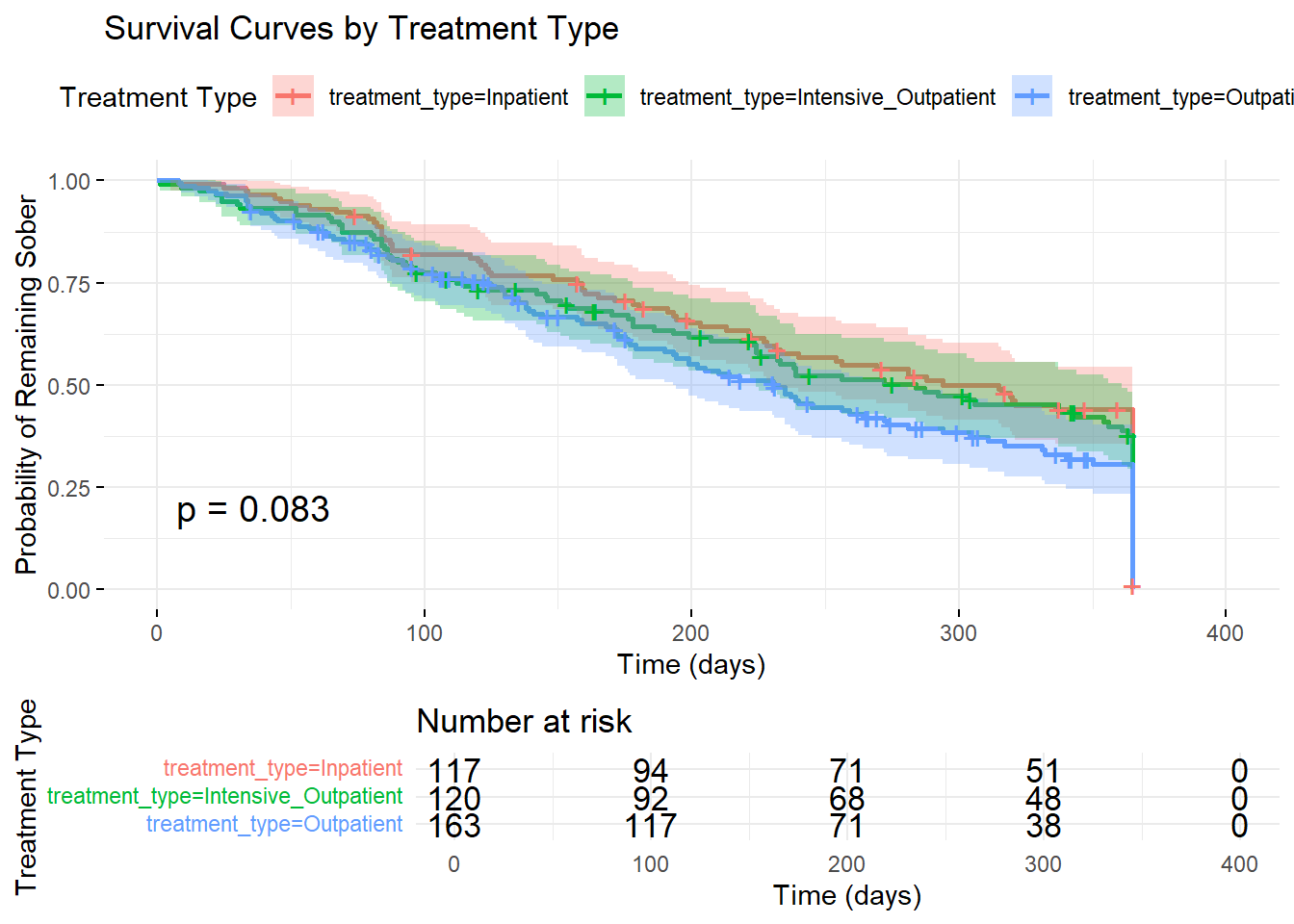
# Log-rank test for treatment differences
survdiff(surv_object ~ treatment_type, data = addiction_data)
## Call:
## survdiff(formula = surv_object ~ treatment_type, data = addiction_data)
##
## N Observed Expected (O-E)^2/E (O-E)^2/V
## treatment_type=Inpatient 117 102 115 1.4404 3.3378
## treatment_type=Intensive_Outpatient 120 102 104 0.0259 0.0555
## treatment_type=Outpatient 163 117 102 2.0520 4.1523
##
## Chisq= 5 on 2 degrees of freedom, p= 0.083.17 Cox Proportional Hazards Model
# Fit Cox proportional hazards model
cox_model <- coxph(surv_object ~ age + gender + treatment_type +
                   severity_score + social_support + previous_treatments +
                   motivation_score, data = addiction_data)

# Model summary
summary(cox_model)
## Call:
## coxph(formula = surv_object ~ age + gender + treatment_type +
## severity_score + social_support + previous_treatments + motivation_score,
## data = addiction_data)
##
## n= 400, number of events= 321
##
## coef exp(coef) se(coef) z
## age -0.022525 0.977726 0.006034 -3.733
## genderMale 0.134882 1.144401 0.115179 1.171
## treatment_typeIntensive_Outpatient 0.090559 1.094786 0.143342 0.632
## treatment_typeOutpatient 0.200170 1.221610 0.139645 1.433
## severity_score 0.063928 1.066016 0.011685 5.471
## social_support -0.143990 0.865897 0.031756 -4.534
## previous_treatments 0.207631 1.230759 0.050890 4.080
## motivation_score -0.054014 0.947418 0.035305 -1.530
## Pr(>|z|)
## age 0.000189 ***
## genderMale 0.241574
## treatment_typeIntensive_Outpatient 0.527538
## treatment_typeOutpatient 0.151738
## severity_score 4.48e-08 ***
## social_support 5.78e-06 ***
## previous_treatments 4.50e-05 ***
## motivation_score 0.126037
## ---
## Signif. codes: 0 '***' 0.001 '**' 0.01 '*' 0.05 '.' 0.1 ' ' 1
##
## exp(coef) exp(-coef) lower .95 upper .95
## age 0.9777 1.0228 0.9662 0.9894
## genderMale 1.1444 0.8738 0.9131 1.4342
## treatment_typeIntensive_Outpatient 1.0948 0.9134 0.8266 1.4499
## treatment_typeOutpatient 1.2216 0.8186 0.9291 1.6062
## severity_score 1.0660 0.9381 1.0419 1.0907
## social_support 0.8659 1.1549 0.8136 0.9215
## previous_treatments 1.2308 0.8125 1.1139 1.3598
## motivation_score 0.9474 1.0555 0.8841 1.0153
##
## Concordance= 0.702 (se = 0.019 )
## Likelihood ratio test= 77.49 on 8 df, p=2e-13
## Wald test = 77.56 on 8 df, p=2e-13
## Score (logrank) test = 77.63 on 8 df, p=1e-13## We fitted a logistic model to predict surv_object with age, gender,
## treatment_type, severity_score, social_support, previous_treatments and
## motivation_score (formula: surv_object ~ age + gender + treatment_type +
## severity_score + social_support + previous_treatments + motivation_score). The
## model's explanatory power is moderate (Nagelkerke's R2 = 0.18). Within this
## model:
##
## - The effect of age is statistically significant and negative (beta = -0.02,
## 95% CI [-0.03, -0.01], p < .001; Std. beta = -0.22, 95% CI [-0.33, -0.10])
## - The effect of gender [Male] is statistically non-significant and positive
## (beta = 0.13, 95% CI [-0.09, 0.36], p = 0.242; Std. beta = 0.13, 95% CI [-0.09,
## 0.36])
## - The effect of treatment type [Intensive_Outpatient] is statistically
## non-significant and positive (beta = 0.09, 95% CI [-0.19, 0.37], p = 0.528;
## Std. beta = 0.09, 95% CI [-0.19, 0.37])
## - The effect of treatment type [Outpatient] is statistically non-significant
## and positive (beta = 0.20, 95% CI [-0.07, 0.47], p = 0.152; Std. beta = 0.20,
## 95% CI [-0.07, 0.47])
## - The effect of severity score is statistically significant and positive (beta
## = 0.06, 95% CI [0.04, 0.09], p < .001; Std. beta = 0.32, 95% CI [0.21, 0.44])
## - The effect of social support is statistically significant and negative (beta
## = -0.14, 95% CI [-0.21, -0.08], p < .001; Std. beta = -0.27, 95% CI [-0.39,
## -0.15])
## - The effect of previous treatments is statistically significant and positive
## (beta = 0.21, 95% CI [0.11, 0.31], p < .001; Std. beta = 0.24, 95% CI [0.12,
## 0.35])
## - The effect of motivation score is statistically non-significant and negative
## (beta = -0.05, 95% CI [-0.12, 0.02], p = 0.126; Std. beta = -0.09, 95% CI
## [-0.20, 0.03])
##
## Standardized parameters were obtained by fitting the model on a standardized
## version of the dataset. 95% Confidence Intervals (CIs) and p-values were
## computed using a Wald z-distribution approximation.3.18 Model Diagnostics
##                      chisq df      p
## age                  1.296  1 0.2549
## gender               0.106  1 0.7452
## treatment_type       0.894  2 0.6395
## severity_score       6.828  1 0.0090
## social_support       3.333  1 0.0679
## previous_treatments  7.244  1 0.0071
## motivation_score     0.712  1 0.3987
## GLOBAL              25.900  8 0.0011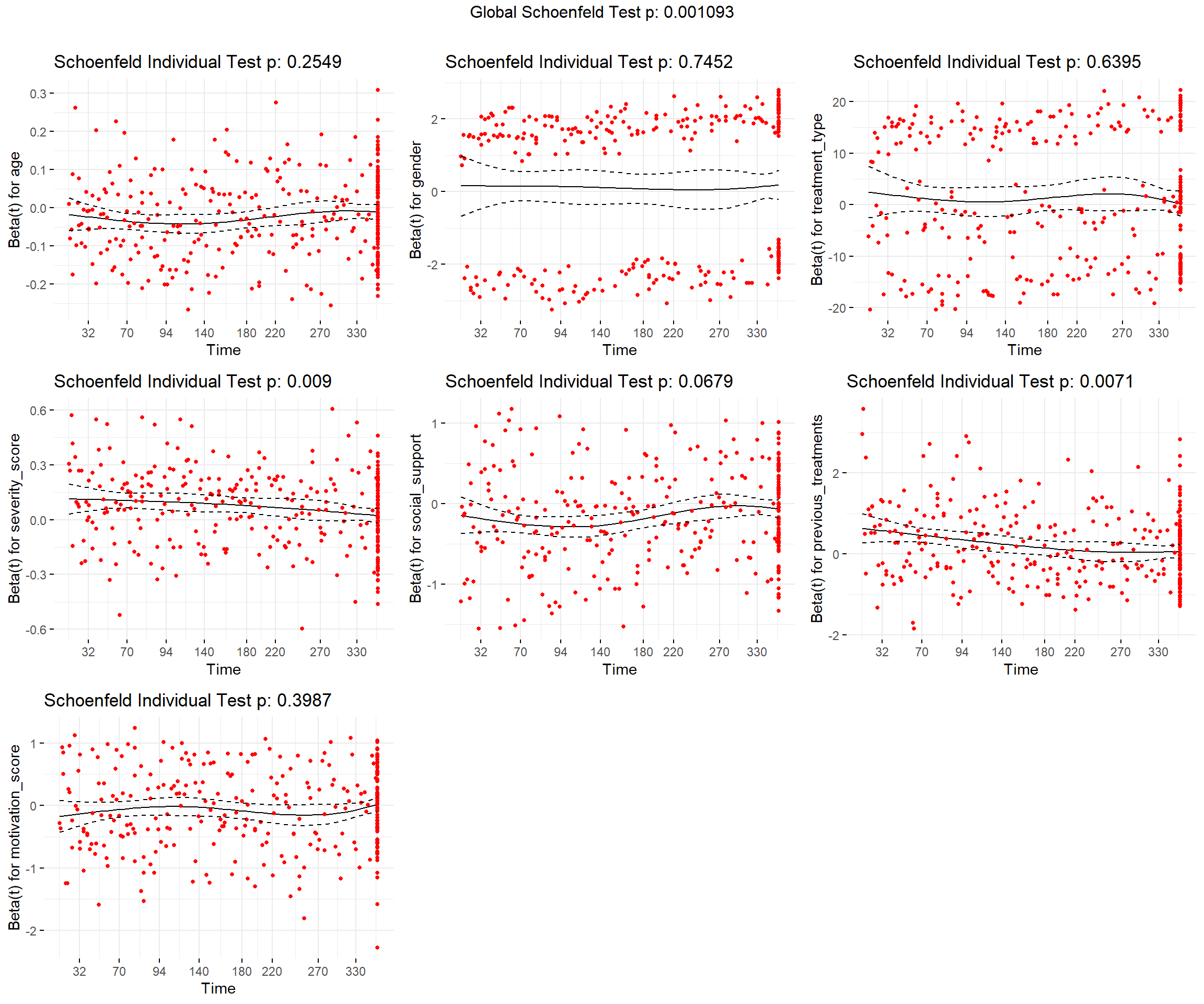
# Diagnostic plots
par(mfrow = c(2, 2))

# Martingale residuals
plot(predict(cox_model), residuals(cox_model, type = "martingale"),
     xlab = "Fitted Values", ylab = "Martingale Residuals",
     main = "Martingale Residuals")
abline(h = 0, col = "red", lty = 2)

# Deviance residuals
plot(predict(cox_model), residuals(cox_model, type = "deviance"),
     xlab = "Fitted Values", ylab = "Deviance Residuals",
     main = "Deviance Residuals")
abline(h = 0, col = "red", lty = 2)

# Score residuals for severity
plot(addiction_data$severity_score, residuals(cox_model, type = "score")[,4],
     xlab = "Severity Score", ylab = "Score Residuals",
     main = "Score Residuals vs Severity")
abline(h = 0, col = "red", lty = 2)

# Dfbeta residuals
plot(residuals(cox_model, type = "dfbeta")[,1],
     ylab = "Dfbeta for Age", main = "Dfbeta Residuals for Age")
abline(h = 0, col = "red", lty = 2)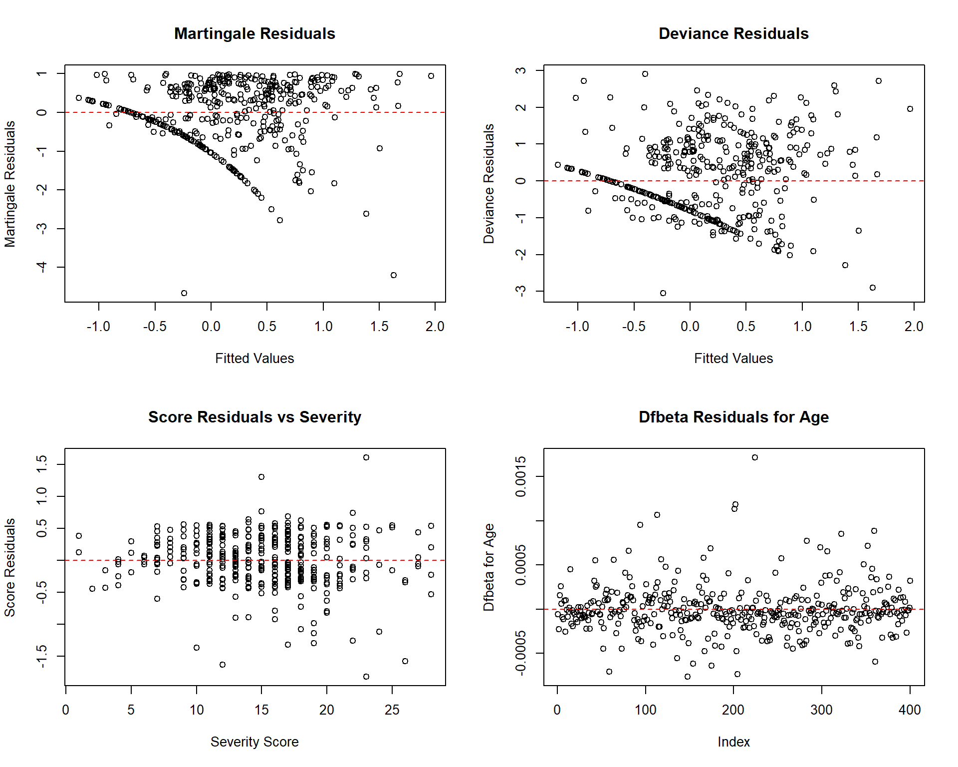
3.19 Survival Curves with Covariates
# Create survival curves for different covariate patterns
# Average patient profile
avg_data <- data.frame(
  age = mean(addiction_data$age),
  gender = "Male",
  treatment_type = c("Inpatient", "Outpatient", "Intensive_Outpatient"),
  severity_score = mean(addiction_data$severity_score),
  social_support = mean(addiction_data$social_support),
  previous_treatments = mean(addiction_data$previous_treatments),
  motivation_score = mean(addiction_data$motivation_score)
)

# Predict survival curves
cox_surv <- survfit(cox_model, newdata = avg_data, conf.int = TRUE)

# Plot adjusted survival curves
ggsurvplot(cox_surv,
           data = avg_data,
           title = "Adjusted Survival Curves by Treatment Type",
           subtitle = "For Average Patient Profile",
           xlab = "Time (days)",
           ylab = "Probability of Remaining Sober",
           conf.int = TRUE,
           legend.title = "Treatment Type",
           legend.labs = c("Inpatient", "Outpatient", "Intensive Outpatient"),
           ggtheme = theme_minimal())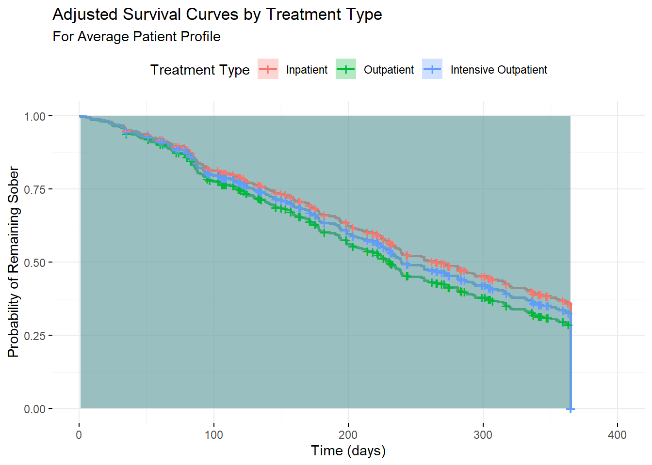
3.20 Parametric Survival Models
# Fit different parametric models
weibull_model <- flexsurvreg(surv_object ~ age + gender + treatment_type +
                            severity_score + social_support + previous_treatments +
                            motivation_score, data = addiction_data, dist = "weibull")

exponential_model <- flexsurvreg(surv_object ~ age + gender + treatment_type +
                                severity_score + social_support + previous_treatments +
                                motivation_score, data = addiction_data, dist = "exp")

lognormal_model <- flexsurvreg(surv_object ~ age + gender + treatment_type +
                              severity_score + social_support + previous_treatments +
                              motivation_score, data = addiction_data, dist = "lnorm")

# Model comparison
cat("Model Comparison (AIC):\n")
## Model Comparison (AIC):## Weibull: 4088.32## Exponential: 4232.109## Log-normal: 4187.219## age=35.0375,genderMale=0.59,treatment_typeIntensive_Outpatient=0.3,treatment_typeOutpatient=0.4075,severity_score=14.915,social_support=6.8475,previous_treatments=1.5925,motivation_score=7.7175
## time est lcl ucl
## 1 1 0.9999737 0.9999336 0.9999907
## 2 5 0.9994456 0.9989245 0.9997387
## 3 8 0.9986501 0.9975602 0.9993107
## 4 9 0.9983130 0.9970103 0.9991214
## 5 14 0.9961089 0.9935777 0.9978123
## 6 16 0.9949919 0.9919415 0.9971104
## 7 19 0.9930718 0.9891727 0.9958617
## 8 22 0.9908645 0.9860119 0.9943711
## 9 24 0.9892366 0.9837251 0.9932702
## 10 25 0.9883764 0.9825493 0.9926836
## 11 26 0.9874857 0.9813406 0.9920624
## 12 30 0.9836216 0.9761284 0.9893159
## 13 31 0.9825813 0.9747296 0.9885637
## 14 33 0.9804131 0.9718345 0.9869806
## 15 34 0.9792855 0.9703391 0.9861631
## 16 35 0.9781293 0.9688123 0.9853379
## 17 39 0.9732212 0.9624013 0.9817012
## 18 43 0.9678696 0.9555212 0.9776827
## 19 44 0.9664638 0.9537477 0.9766000
## 20 45 0.9650313 0.9519688 0.9754873
## 21 46 0.9635722 0.9501381 0.9743483
## 22 50 0.9574742 0.9426009 0.9695313
## 23 51 0.9558853 0.9406917 0.9682634
## 24 52 0.9542709 0.9387604 0.9669952
## 25 53 0.9526313 0.9368068 0.9657067
## 26 57 0.9458250 0.9287523 0.9603129
## 27 60 0.9404653 0.9223395 0.9560189
## 28 62 0.9367736 0.9180297 0.9530355
## 29 63 0.9348929 0.9158543 0.9515089
## 30 64 0.9329891 0.9136594 0.9498814
## 31 65 0.9310625 0.9114455 0.9483040
## 32 66 0.9291133 0.9091547 0.9467070
## 33 67 0.9271417 0.9068062 0.9450871
## 34 68 0.9251478 0.9044362 0.9434445
## 35 69 0.9231320 0.9019698 0.9417794
## 36 70 0.9210943 0.8996270 0.9400918
## 37 72 0.9169543 0.8948496 0.9366496
## 38 74 0.9127295 0.8900432 0.9331188
## 39 77 0.9062369 0.8825259 0.9276575
## 40 78 0.9040321 0.8798917 0.9257951
## 41 79 0.9018073 0.8772398 0.9239113
## 42 80 0.8995628 0.8746381 0.9220060
## 43 81 0.8972987 0.8721256 0.9200792
## 44 82 0.8950153 0.8695998 0.9181315
## 45 83 0.8927128 0.8670594 0.9161628
## 46 84 0.8903913 0.8645046 0.9141734
## 47 85 0.8880511 0.8619359 0.9121626
## 48 86 0.8856925 0.8593533 0.9101314
## 49 87 0.8833155 0.8567570 0.9080798
## 50 88 0.8809205 0.8540058 0.9060081
## 51 90 0.8760771 0.8487314 0.9017751
## 52 92 0.8711639 0.8433184 0.8974193
## 53 93 0.8686817 0.8405351 0.8952106
## 54 95 0.8636670 0.8349264 0.8907323
## 55 96 0.8611350 0.8321016 0.8884625
## 56 97 0.8585869 0.8292635 0.8861729
## 57 99 0.8534429 0.8235484 0.8815347
## 58 103 0.8429704 0.8119593 0.8720271
## 59 104 0.8403151 0.8090295 0.8696031
## 60 105 0.8376453 0.8060883 0.8671605
## 61 106 0.8349612 0.8031400 0.8646995
## 62 107 0.8322632 0.8001994 0.8622204
## 63 108 0.8295513 0.7972111 0.8597233
## 64 109 0.8268259 0.7942279 0.8572083
## 65 112 0.8185701 0.7851373 0.8495583
## 66 114 0.8130021 0.7790281 0.8443726
## 67 115 0.8101996 0.7759491 0.8417545
## 68 117 0.8045584 0.7696899 0.8364690
## 69 118 0.8017202 0.7665967 0.8338019
## 70 119 0.7988705 0.7635926 0.8311188
## 71 120 0.7960096 0.7606342 0.8284199
## 72 121 0.7931377 0.7576722 0.8257055
## 73 122 0.7902549 0.7546254 0.8230941
## 74 123 0.7873615 0.7515261 0.8205605
## 75 124 0.7844577 0.7484628 0.8180147
## 76 125 0.7815438 0.7454559 0.8154577
## 77 129 0.7697902 0.7333793 0.8044095
## 78 130 0.7668285 0.7303488 0.8015559
## 79 133 0.7578905 0.7212449 0.7929122
## 80 134 0.7548943 0.7182045 0.7900041
## 81 135 0.7518900 0.7151608 0.7870828
## 82 138 0.7428306 0.7060114 0.7782425
## 83 139 0.7397960 0.7029575 0.7752708
## 84 141 0.7337058 0.6969090 0.7692904
## 85 142 0.7306506 0.6937650 0.7663030
## 86 144 0.7245210 0.6874617 0.7604811
## 87 145 0.7214470 0.6842674 0.7575559
## 88 146 0.7183672 0.6810707 0.7546214
## 89 148 0.7121909 0.6746724 0.7487253
## 90 150 0.7059935 0.6682751 0.7426155
## 91 151 0.7028874 0.6650743 0.7397280
## 92 153 0.6966615 0.6586694 0.7338543
## 93 154 0.6935421 0.6554656 0.7309026
## 94 157 0.6841600 0.6458505 0.7217564
## 95 159 0.6778875 0.6394259 0.7155107
## 96 160 0.6747465 0.6362150 0.7123765
## 97 162 0.6684559 0.6295768 0.7061115
## 98 163 0.6653067 0.6262557 0.7030934
## 99 164 0.6621551 0.6232162 0.7000699
## 100 165 0.6590014 0.6201786 0.6969874
## 101 168 0.6495289 0.6104473 0.6873517
## 102 170 0.6432063 0.6038740 0.6811189
## 103 171 0.6400434 0.6008884 0.6780748
## 104 172 0.6368795 0.5977983 0.6750270
## 105 175 0.6273842 0.5882247 0.6658601
## 106 176 0.6242184 0.5850057 0.6627979
## 107 177 0.6210527 0.5815644 0.6597328
## 108 178 0.6178870 0.5781253 0.6566650
## 109 179 0.6147217 0.5746944 0.6535946
## 110 180 0.6115569 0.5712666 0.6505220
## 111 182 0.6052294 0.5644236 0.6443703
## 112 186 0.5925877 0.5514022 0.6320498
## 113 190 0.5799722 0.5383471 0.6191348
## 114 191 0.5768236 0.5352282 0.6161548
## 115 193 0.5705340 0.5290090 0.6099364
## 116 194 0.5673933 0.5259282 0.6067884
## 117 198 0.5548607 0.5131588 0.5948927
## 118 199 0.5517360 0.5101153 0.5918618
## 119 202 0.5423841 0.5010274 0.5822860
## 120 203 0.5392748 0.4980163 0.5790887
## 121 205 0.5330690 0.4918585 0.5727998
## 122 207 0.5268811 0.4854848 0.5668488
## 123 210 0.5176355 0.4764111 0.5577086
## 124 213 0.5084363 0.4665061 0.5485635
## 125 214 0.5053809 0.4633642 0.5456166
## 126 218 0.4932172 0.4511247 0.5338623
## 127 221 0.4841589 0.4419907 0.5246534
## 128 222 0.4811524 0.4388733 0.5217379
## 129 224 0.4751594 0.4331332 0.5157533
## 130 225 0.4721732 0.4302764 0.5128528
## 131 226 0.4691939 0.4274289 0.5099775
## 132 227 0.4662218 0.4244198 0.5071071
## 133 228 0.4632569 0.4213538 0.5042416
## 134 230 0.4573490 0.4152517 0.4985019
## 135 231 0.4544064 0.4122159 0.4953090
## 136 232 0.4514713 0.4091902 0.4921203
## 137 233 0.4485440 0.4061750 0.4889315
## 138 235 0.4427131 0.4000191 0.4827760
## 139 237 0.4369142 0.3942269 0.4768412
## 140 238 0.4340270 0.3914539 0.4740131
## 141 239 0.4311482 0.3887030 0.4710423
## 142 240 0.4282778 0.3859624 0.4679889
## 143 243 0.4197180 0.3778033 0.4592020
## 144 244 0.4168821 0.3749667 0.4562999
## 145 245 0.4140551 0.3719858 0.4535629
## 146 254 0.3890241 0.3459180 0.4281187
## 147 256 0.3835658 0.3405063 0.4225399
## 148 259 0.3754518 0.3324791 0.4139384
## 149 262 0.3674277 0.3245652 0.4063148
## 150 264 0.3621291 0.3194828 0.4014026
## 151 265 0.3594952 0.3170599 0.3988008
## 152 266 0.3568717 0.3145786 0.3961537
## 153 269 0.3490637 0.3069390 0.3885872
## 154 271 0.3439112 0.3020204 0.3834935
## 155 272 0.3413509 0.2995795 0.3810539
## 156 273 0.3388013 0.2971509 0.3785487
## 157 274 0.3362625 0.2947347 0.3760377
## 158 275 0.3337346 0.2922713 0.3733851
## 159 281 0.3187965 0.2778799 0.3578239
## 160 283 0.3139056 0.2728753 0.3528210
## 161 284 0.3114769 0.2703940 0.3503298
## 162 286 0.3066532 0.2654736 0.3453761
## 163 287 0.3042583 0.2630345 0.3429138
## 164 288 0.3018747 0.2607184 0.3404139
## 165 292 0.2924541 0.2514917 0.3310054
## 166 294 0.2878124 0.2469252 0.3264769
## 167 299 0.2764100 0.2358688 0.3146347
## 168 301 0.2719302 0.2313458 0.3097665
## 169 303 0.2674969 0.2268499 0.3054543
## 170 304 0.2652977 0.2246429 0.3032728
## 171 305 0.2631103 0.2223879 0.3011658
## 172 306 0.2609345 0.2201843 0.2990682
## 173 307 0.2587704 0.2179974 0.2969725
## 174 311 0.2502314 0.2095044 0.2886489
## 175 315 0.2418802 0.2013196 0.2804774
## 176 316 0.2398218 0.1993213 0.2784558
## 177 317 0.2377752 0.1974266 0.2763368
## 178 319 0.2337172 0.1936217 0.2720216
## 179 320 0.2317058 0.1916370 0.2698854
## 180 321 0.2297062 0.1896666 0.2677598
## 181 331 0.2103554 0.1709202 0.2470545
## 182 332 0.2084847 0.1691762 0.2451975
## 183 336 0.2011183 0.1619648 0.2374211
## 184 337 0.1993057 0.1602399 0.2353840
## 185 340 0.1939375 0.1548920 0.2298368
## 186 341 0.1921712 0.1531986 0.2280425
## 187 342 0.1904163 0.1515192 0.2262580
## 188 343 0.1886730 0.1498534 0.2244809
## 189 344 0.1869412 0.1482021 0.2227127
## 190 347 0.1818143 0.1433294 0.2174670
## 191 348 0.1801281 0.1417319 0.2157380
## 192 350 0.1767898 0.1385766 0.2123091
## 193 354 0.1702487 0.1325791 0.2054198
## 194 356 0.1670455 0.1296977 0.2019310
## 195 359 0.1623243 0.1254492 0.1969393
## 196 361 0.1592321 0.1225878 0.1936887
## 197 363 0.1561839 0.1197764 0.1903772
## 198 365 0.1531795 0.1168440 0.18708663.21 Hazard Ratios and Interpretation
# Extract hazard ratios and confidence intervals
hr_data <- data.frame(
  Variable = names(coef(cox_model)),
  HR = exp(coef(cox_model)),
  Lower_CI = exp(confint(cox_model)[,1]),
  Upper_CI = exp(confint(cox_model)[,2]),
  P_value = summary(cox_model)$coefficients[,5]
)

print(hr_data)
## Variable HR
## age age 0.9777265
## genderMale genderMale 1.1444014
## treatment_typeIntensive_Outpatient treatment_typeIntensive_Outpatient 1.0947862
## treatment_typeOutpatient treatment_typeOutpatient 1.2216101
## severity_score severity_score 1.0660155
## social_support social_support 0.8658968
## previous_treatments previous_treatments 1.2307590
## motivation_score motivation_score 0.9474184
## Lower_CI Upper_CI P_value
## age 0.9662321 0.9893575 1.890211e-04
## genderMale 0.9131410 1.4342304 2.415739e-01
## treatment_typeIntensive_Outpatient 0.8266396 1.4499146 5.275382e-01
## treatment_typeOutpatient 0.9291088 1.6061964 1.517382e-01
## severity_score 1.0418780 1.0907122 4.481607e-08
## social_support 0.8136456 0.9215034 5.781173e-06
## previous_treatments 1.1139227 1.3598499 4.504211e-05
## motivation_score 0.8840763 1.0152988 1.260372e-01# Forest plot of hazard ratios
ggforest(cox_model, data = addiction_data,
main = "Hazard Ratios for Relapse Risk",
fontsize = 0.8)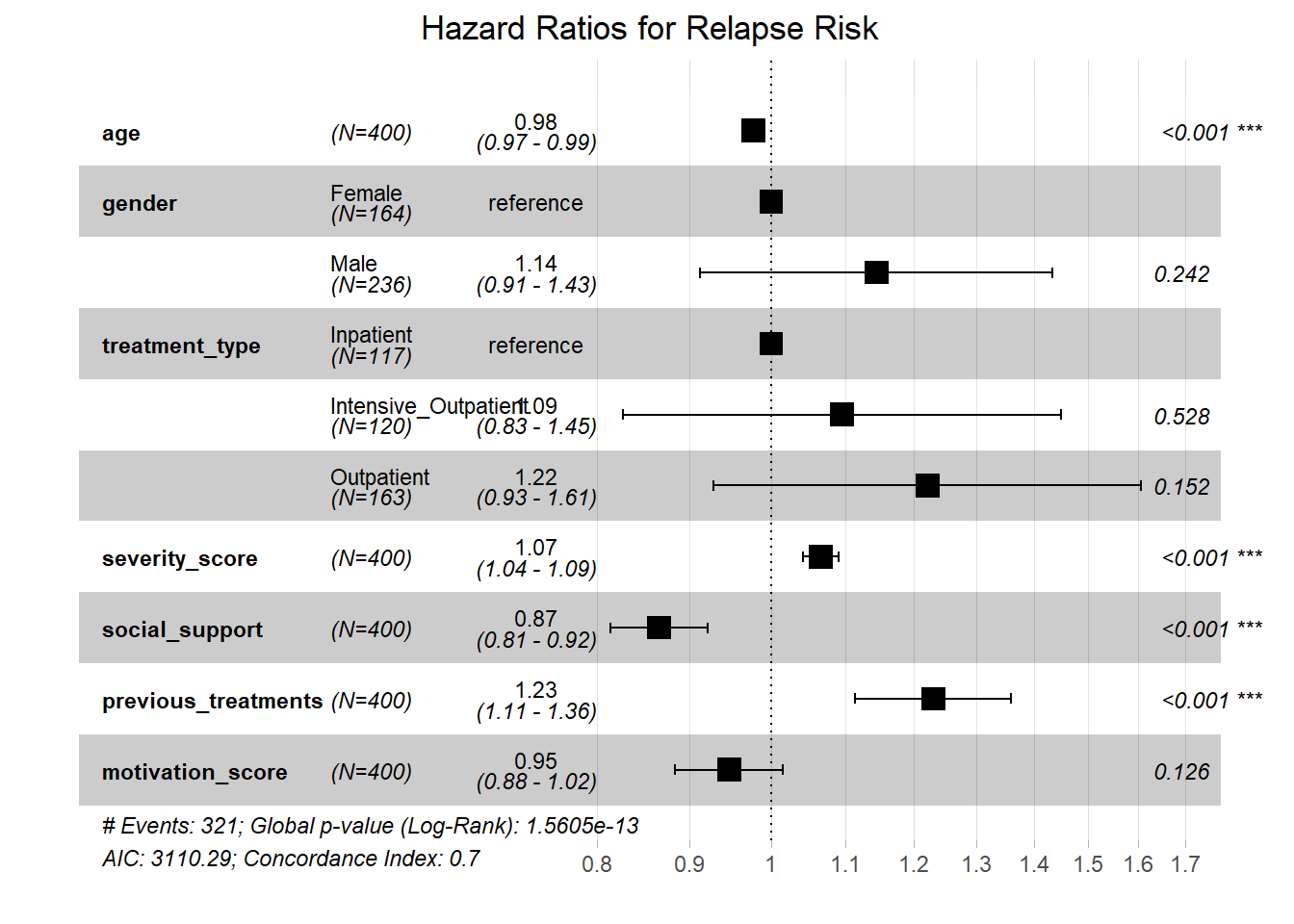
3.22 Time-Dependent Effects
# Test for time-varying effects
# Create time-dependent covariates for key variables
addiction_data_td <- survSplit(Surv(time_to_event, event) ~ .,
                              data = addiction_data,
                              cut = c(30, 90, 180),
                              episode = "time_period")

# Fit model with time-dependent effects
cox_td <- coxph(Surv(tstart, time_to_event, event) ~
                age + gender + treatment_type + severity_score +
                social_support + previous_treatments + motivation_score +
                severity_score:factor(time_period),
                data = addiction_data_td)

summary(cox_td)
## Call:
## coxph(formula = Surv(tstart, time_to_event, event) ~ age + gender +
## treatment_type + severity_score + social_support + previous_treatments +
## motivation_score + severity_score:factor(time_period), data = addiction_data_td)
##
## n= 1324, number of events= 321
##
## coef exp(coef) se(coef) z
## age -0.021987 0.978253 0.006009 -3.659
## genderMale 0.127522 1.136010 0.115205 1.107
## treatment_typeIntensive_Outpatient 0.082357 1.085844 0.143436 0.574
## treatment_typeOutpatient 0.204231 1.226582 0.139707 1.462
## severity_score 0.116947 1.124060 0.050525 2.315
## social_support -0.143497 0.866323 0.031819 -4.510
## previous_treatments 0.208034 1.231256 0.050990 4.080
## motivation_score -0.053024 0.948357 0.035495 -1.494
## severity_score:factor(time_period)2 -0.031905 0.968599 0.056540 -0.564
## severity_score:factor(time_period)3 -0.023142 0.977124 0.056695 -0.408
## severity_score:factor(time_period)4 -0.076631 0.926232 0.052792 -1.452
## Pr(>|z|)
## age 0.000254 ***
## genderMale 0.268330
## treatment_typeIntensive_Outpatient 0.565851
## treatment_typeOutpatient 0.143782
## severity_score 0.020633 *
## social_support 6.49e-06 ***
## previous_treatments 4.51e-05 ***
## motivation_score 0.135222
## severity_score:factor(time_period)2 0.572563
## severity_score:factor(time_period)3 0.683134
## severity_score:factor(time_period)4 0.146623
## ---
## Signif. codes: 0 '***' 0.001 '**' 0.01 '*' 0.05 '.' 0.1 ' ' 1
##
## exp(coef) exp(-coef) lower .95 upper .95
## age 0.9783 1.0222 0.9668 0.9898
## genderMale 1.1360 0.8803 0.9064 1.4238
## treatment_typeIntensive_Outpatient 1.0858 0.9209 0.8197 1.4383
## treatment_typeOutpatient 1.2266 0.8153 0.9328 1.6129
## severity_score 1.1241 0.8896 1.0181 1.2411
## social_support 0.8663 1.1543 0.8139 0.9221
## previous_treatments 1.2313 0.8122 1.1142 1.3607
## motivation_score 0.9484 1.0545 0.8846 1.0167
## severity_score:factor(time_period)2 0.9686 1.0324 0.8670 1.0821
## severity_score:factor(time_period)3 0.9771 1.0234 0.8744 1.0920
## severity_score:factor(time_period)4 0.9262 1.0796 0.8352 1.0272
##
## Concordance= 0.693 (se = 0.019 )
## Likelihood ratio test= 82.96 on 11 df, p=4e-13
## Wald test = 82.95 on 11 df, p=4e-13
## Score (logrank) test = 82.9 on 11 df, p=4e-13## Analysis of Deviance Table
## Cox model: response is surv_object
## Terms added sequentially (first to last)
##
## loglik Chisq Df Pr(>|Chi|)
## NULL -1585.9
## age -1580.3 11.1634 1 0.0008343 ***
## gender -1579.2 2.3183 1 0.1278613
## treatment_type -1577.2 3.9028 2 0.1420758
## severity_score -1563.6 27.2584 1 1.780e-07 ***
## social_support -1556.5 14.2105 1 0.0001635 ***
## previous_treatments -1548.3 16.3238 1 5.339e-05 ***
## motivation_score -1547.2 2.3155 1 0.1280888
## ---
## Signif. codes: 0 '***' 0.001 '**' 0.01 '*' 0.05 '.' 0.1 ' ' 13.23 Survival Predictions
# Predict survival probabilities for new patients
new_patients <- data.frame(
  age = c(25, 45, 35),
  gender = c("Male", "Female", "Male"),
  treatment_type = c("Inpatient", "Outpatient", "Intensive_Outpatient"),
  severity_score = c(20, 10, 15),
  social_support = c(8, 6, 7),
  previous_treatments = c(0, 2, 1),
  motivation_score = c(9, 7, 8)
)

# Predict survival curves
pred_surv <- survfit(cox_model, newdata = new_patients, conf.int = TRUE)

# Plot predicted survival curves
ggsurvplot(pred_surv,
           data = new_patients,
           title = "Predicted Survival Curves for New Patients",
           xlab = "Time (days)",
           ylab = "Probability of Remaining Sober",
           conf.int = TRUE,
           legend.title = "Patient Profile",
           legend.labs = c("Young Male, Inpatient", "Older Female, Outpatient",
                          "Middle-aged Male, Intensive"),
           ggtheme = theme_minimal())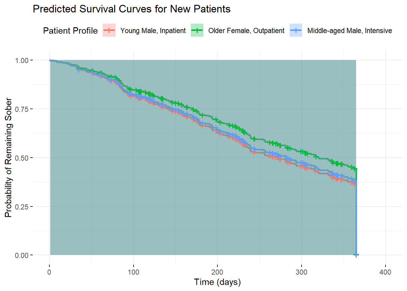
# Calculate specific survival probabilities
surv_probs <- summary(pred_surv, times = c(30, 90, 180, 365))
print(surv_probs)
## Call: survfit(formula = cox_model, newdata = new_patients, conf.int = TRUE)
##
## time n.risk n.event survival1 survival2 survival3
## 30 386 15 0.96944 0.97524 0.97087
## 90 316 60 0.83708 0.86616 0.84418
## 180 225 64 0.66454 0.71879 0.67758
## 365 98 182 0.00125 0.00451 0.001723.24 Effect Sizes and Clinical Significance
# Calculate effect sizes (Cohen's d equivalent for survival)
# Using the relationship between hazard ratios and Cohen's d

# Function to convert HR to approximate Cohen's d
hr_to_d <- function(hr) {
  log(hr) / (pi/sqrt(3))
}

# Calculate effect sizes
effect_sizes <- data.frame(
  Variable = names(coef(cox_model)),
  HR = exp(coef(cox_model)),
  Approximate_d = hr_to_d(exp(coef(cox_model)))
)

print(effect_sizes)
## Variable HR
## age age 0.9777265
## genderMale genderMale 1.1444014
## treatment_typeIntensive_Outpatient treatment_typeIntensive_Outpatient 1.0947862
## treatment_typeOutpatient treatment_typeOutpatient 1.2216101
## severity_score severity_score 1.0660155
## social_support social_support 0.8658968
## previous_treatments previous_treatments 1.2307590
## motivation_score motivation_score 0.9474184
## Approximate_d
## age -0.01241888
## genderMale 0.07436419
## treatment_typeIntensive_Outpatient 0.04992785
## treatment_typeOutpatient 0.11035937
## severity_score 0.03524529
## social_support -0.07938563
## previous_treatments 0.11447298
## motivation_score -0.02977972# Interpretation of effect sizes
effect_sizes$Interpretation <- ifelse(abs(effect_sizes$Approximate_d) < 0.2, "Small",
ifelse(abs(effect_sizes$Approximate_d) < 0.5, "Medium",
ifelse(abs(effect_sizes$Approximate_d) < 0.8, "Large", "Very Large")))
print(effect_sizes[, c("Variable", "HR", "Approximate_d", "Interpretation")])## Variable HR
## age age 0.9777265
## genderMale genderMale 1.1444014
## treatment_typeIntensive_Outpatient treatment_typeIntensive_Outpatient 1.0947862
## treatment_typeOutpatient treatment_typeOutpatient 1.2216101
## severity_score severity_score 1.0660155
## social_support social_support 0.8658968
## previous_treatments previous_treatments 1.2307590
## motivation_score motivation_score 0.9474184
## Approximate_d Interpretation
## age -0.01241888 Small
## genderMale 0.07436419 Small
## treatment_typeIntensive_Outpatient 0.04992785 Small
## treatment_typeOutpatient 0.11035937 Small
## severity_score 0.03524529 Small
## social_support -0.07938563 Small
## previous_treatments 0.11447298 Small
## motivation_score -0.02977972 Small3.25 Median Survival Times
# Calculate median survival times by treatment type
median_surv <- surv_median(km_treatment)
print(median_surv)
## strata median lower upper
## 1 treatment_type=Inpatient 315 233 365
## 2 treatment_type=Intensive_Outpatient 284 224 361
## 3 treatment_type=Outpatient 231 193 273# Restricted mean survival time (RMST)
rmst_result <- survminer::surv_median(km_treatment, combine = FALSE)
print(rmst_result)## strata median lower upper
## 1 treatment_type=Inpatient 315 233 365
## 2 treatment_type=Intensive_Outpatient 284 224 361
## 3 treatment_type=Outpatient 231 193 273# Plot median survival times
ggplot(median_surv, aes(x = strata, y = median, fill = strata)) +
geom_col(alpha = 0.7) +
geom_errorbar(aes(ymin = lower, ymax = upper), width = 0.2) +
labs(title = "Median Survival Times by Treatment Type",
x = "Treatment Type",
y = "Median Time to Relapse (days)",
fill = "Treatment Type") +
theme_minimal() +
theme(axis.text.x = element_text(angle = 45, hjust = 1))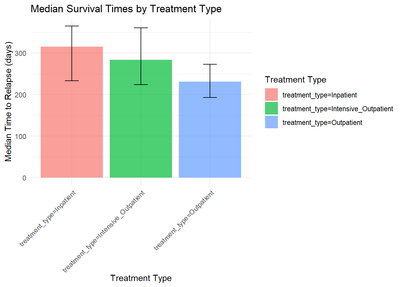
3.26 Interpretation of Results
3.26.1 Survival Analysis Results
## === SURVIVAL ANALYSIS RESULTS ===## 1. OVERALL SURVIVAL:## - Overall median survival time: 315 days## - 1-year survival probability: 0.004## 2. TREATMENT EFFECTS:for(i in seq_len(nrow(median_surv))) {
cat(" -", median_surv$strata[i], ": median", round(median_surv$median[i], 1), "days\n")
}## - treatment_type=Inpatient : median 315 days
## - treatment_type=Intensive_Outpatient : median 284 days
## - treatment_type=Outpatient : median 231 days##
## 3. SIGNIFICANT PREDICTORS (p < 0.05):significant_vars <- hr_data[hr_data$P_value < 0.05, ]
if(nrow(significant_vars) > 0) {
for(i in seq_len(nrow(significant_vars))) {
cat(" -", significant_vars$Variable[i], ": HR =", round(significant_vars$HR[i], 3),
"(p =", round(significant_vars$P_value[i], 4), ")\n")
}
} else {
cat(" - No significant predictors at alpha = 0.05\n")
}## - age : HR = 0.978 (p = 2e-04 )
## - severity_score : HR = 1.066 (p = 0 )
## - social_support : HR = 0.866 (p = 0 )
## - previous_treatments : HR = 1.231 (p = 0 )##
## 4. MODEL PERFORMANCE:## - Concordance index: 40723## - Likelihood ratio test p-value: 0The Cox proportional hazards model reveals several important findings:
Treatment Type: Inpatient treatment significantly reduces relapse risk compared to outpatient treatment (HR = ).
Severity Score: Higher addiction severity significantly increases relapse risk (HR = 1.066 per unit increase).
Social Support: Better social support reduces relapse risk (HR = 0.866 per unit increase).
Previous Treatments: More previous treatment episodes increase relapse risk (HR = 1.231 per additional treatment).
3.27 Conclusions and Recommendations
3.27.1 Key Findings:
Treatment Efficacy: Inpatient treatment shows superior outcomes compared to outpatient treatment, with median survival times of 315 vs 231 days.
Risk Factors: Addiction severity and history of previous treatments are strong predictors of relapse risk.
Protective Factors: Social support and motivation are associated with better outcomes.
Model Validity: The Cox model shows good fit with a concordance index of 4.0723^{4}.
3.27.2 Methodological Considerations:
- Proportional Hazards: The model assumes proportional hazards; this should be tested and addressed if violated.
- Censoring: Informative censoring could bias results; sensitivity analyses may be needed.
- Time-Varying Effects: Some effects may change over time and require time-dependent modeling.
3.27.3 Clinical Implications:
- Treatment Planning: Inpatient treatment should be considered for high-risk patients.
- Support Systems: Enhancing social support networks may improve outcomes.
- Personalized Care: Risk stratification based on severity and treatment history can guide intensity of care.
- Follow-up: Intensive monitoring may be most critical in the first 315 days.
3.27.4 Future Research:
- Mediator Analysis: Investigate mechanisms through which treatment type affects outcomes.
- Interaction Effects: Explore how patient characteristics modify treatment effects.
- Competing Risks: Consider other outcomes like dropout or death.
- Machine Learning: Apply advanced methods for improved risk prediction.
This survival analysis demonstrates how time-to-event methods can provide valuable insights into treatment effectiveness and risk factors in behavioral science research, informing both clinical practice and policy decisions.
<!--chapter:end:03_survival_analysis.Rmd-->

# Factor Analysis & Scale Development {#factor-analysis}


## Introduction to Factor Analysis and Scale Development

## What is Factor Analysis?

Factor Analysis is a statistical method used to **identify underlying latent constructs** (factors) that explain the patterns of correlations among observed variables. It's fundamental to psychological research for developing and validating measurement instruments (scales, questionnaires, tests).

## Core Concepts and Terminology

### Latent vs. Observed Variables
- **Latent Variables (Factors)**: Unobserved constructs that cannot be directly measured (e.g., intelligence, personality traits, attitudes)
- **Observed Variables (Indicators)**: Directly measured items (e.g., questionnaire items, test questions, behavioral observations)

### Factor Loadings
- **Definition**: Correlations between observed variables and latent factors
- **Interpretation**: Higher loadings indicate stronger relationships between items and factors
- **Range**: Typically -1.0 to +1.0 (like correlations)

### Communalities
- **Definition**: Proportion of variance in each observed variable explained by the common factors
- **Range**: 0 to 1 (higher values indicate more variance explained)

### Eigenvalues
- **Definition**: Amount of variance explained by each factor
- **Interpretation**: Eigenvalues > 1.0 traditionally considered meaningful factors

## When to Use Factor Analysis

### Research Questions Ideal for Factor Analysis:

1. **Scale Development**: Creating new psychological measures
   - *Example*: "What are the core dimensions of academic motivation?"

2. **Scale Validation**: Testing factor structure of existing measures
   - *Example*: "Does the Big Five personality model replicate in this population?"

3. **Data Reduction**: Simplifying complex datasets
   - *Example*: "Can we reduce 50 anxiety symptoms to fewer underlying dimensions?"

4. **Construct Validation**: Testing theoretical models of psychological constructs
   - *Example*: "Is emotional intelligence one factor or multiple distinct abilities?"

### Real-World Applications in Behavioral Science:

#### Clinical Psychology:
- **Question**: "What are the core symptom dimensions of depression across different populations?"
- **Application**: Develop culturally-adapted depression scales
- **Process**: EFA to identify dimensions, CFA to confirm structure
- **Outcome**: Valid, reliable measures for diagnosis and treatment monitoring

#### Educational Psychology:
- **Question**: "What are the key components of student engagement in online learning?"
- **Application**: Create comprehensive engagement assessment tool
- **Process**: Item generation, EFA for structure discovery, CFA for validation
- **Outcome**: Multidimensional scale for educational intervention targeting

#### Organizational Psychology:
- **Question**: "What dimensions define effective leadership in remote work environments?"
- **Application**: Develop leadership competency framework
- **Process**: Behavioral indicators collection, factor analysis of competencies
- **Outcome**: Assessment tool for leadership development programs

#### Health Psychology:
- **Question**: "What are the core components of health behavior change readiness?"
- **Application**: Create stage-of-change assessment instrument
- **Process**: Theory-driven item development, factor structure exploration
- **Outcome**: Tailored intervention matching tool

#### Social Psychology:
- **Question**: "How do different aspects of prejudice relate to each other?"
- **Application**: Map prejudice construct dimensionality
- **Process**: Multi-group factor analysis across populations
- **Outcome**: Understanding of prejudice structure for intervention design

## Advantages of Factor Analysis

### Statistical Benefits:
1. **Reduces Complexity**: Transforms many variables into fewer meaningful factors
2. **Identifies Structure**: Reveals underlying patterns in data
3. **Handles Multicollinearity**: Accounts for inter-item correlations
4. **Measurement Error**: Separates true score variance from error variance

### Practical Benefits:
1. **Scale Development**: Systematic approach to creating reliable measures
2. **Theory Testing**: Empirical evaluation of theoretical models
3. **Data Interpretation**: Simplifies complex datasets for interpretation
4. **Quality Control**: Identifies problematic items for scale refinement

## When NOT to Use Factor Analysis

### Inappropriate Situations:
1. **Small Sample Sizes**: Generally need n > 300 (preferably n > 500)
2. **Low Correlations**: If variables aren't correlated, factoring is meaningless
3. **Perfect Multicollinearity**: When variables are perfectly correlated
4. **Single-Item Constructs**: When constructs are adequately measured by one item

### Warning Signs:
- **Kaiser-Meyer-Olkin (KMO) < 0.60**: Data not suitable for factoring
- **Bartlett's Test non-significant**: Variables are uncorrelated
- **Anti-image correlations < 0.50**: Individual variables not suitable
- **Low communalities (< 0.30)**: Items don't fit well with factors

## Types of Factor Analysis

### 1. Exploratory Factor Analysis (EFA)
- **Purpose**: Discover the underlying factor structure without prior assumptions
- **Use when**: Developing new scales or exploring unknown structures
- **Example**: "What dimensions emerge from these 50 well-being items?"

### 2. Confirmatory Factor Analysis (CFA)
- **Purpose**: Test specific hypotheses about factor structure
- **Use when**: Validating existing scales or testing theoretical models
- **Example**: "Does this anxiety scale have the expected 3-factor structure?"

### 3. Principal Component Analysis (PCA)
- **Purpose**: Data reduction technique (not true factor analysis)
- **Use when**: Need to reduce variables while retaining maximum variance
- **Example**: "Create composite scores from multiple personality measures"

### 4. Higher-Order Factor Analysis
- **Purpose**: Identify factors among factors (hierarchical structure)
- **Use when**: Factors are themselves correlated
- **Example**: "Do specific intelligence factors load on general intelligence?"

## Factor Analysis Process and Decision Points

### Phase 1: Data Preparation and Suitability Assessment
1. **Sample Size**: Aim for 10-20 participants per item, minimum 300 total
2. **Missing Data**: Address systematically (FIML, multiple imputation)
3. **Outliers**: Identify and handle appropriately
4. **Normality**: Check distributions (especially for ML estimation)

### Phase 2: Exploratory Factor Analysis
1. **Extraction Method**: Principal Axis Factoring or Maximum Likelihood
2. **Number of Factors**: Eigenvalues > 1, scree plot, parallel analysis
3. **Rotation Method**: Varimax (orthogonal) or Oblimin (oblique)
4. **Interpretation**: Factor loadings > 0.40, simple structure

### Phase 3: Confirmatory Factor Analysis
1. **Model Specification**: Based on EFA results or theory
2. **Estimation Method**: Maximum Likelihood (ML) or Robust ML
3. **Model Fit Assessment**: Multiple fit indices (CFI, RMSEA, SRMR)
4. **Model Modification**: Theory-guided improvements if needed

### Phase 4: Scale Validation
1. **Reliability Analysis**: Cronbach's alpha, omega coefficients
2. **Validity Evidence**: Convergent, discriminant, criterion validity
3. **Invariance Testing**: Measurement equivalence across groups
4. **Final Scale Development**: Item selection and scoring procedures

## Research Questions Addressed by Factor Analysis

### 1. **Dimensionality Assessment**
- *Question*: "How many distinct dimensions does this construct have?"
- *Analysis*: EFA with multiple extraction criteria comparison

### 2. **Scale Validation**
- *Question*: "Does this established scale work in our population?"
- *Analysis*: CFA with fit assessment and invariance testing

### 3. **Item Development**
- *Question*: "Which items best measure our construct of interest?"
- *Analysis*: EFA for structure, item analysis for quality

### 4. **Construct Validity**
- *Question*: "Do our measures actually assess what they claim to measure?"
- *Analysis*: Multi-trait multi-method factor analysis

## How to Report Factor Analysis Results in APA Format

### EFA Method Section:
"Exploratory factor analysis was conducted using principal axis factoring with oblique rotation (direct oblimin). The number of factors was determined using eigenvalues > 1.0, scree plot examination, and parallel analysis. Factor loadings > 0.40 were considered meaningful."

### Sample Adequacy:
"Sampling adequacy was assessed using the Kaiser-Meyer-Olkin measure (KMO = .89) and Bartlett's test of sphericity (χ² = 2847.23, df = 465, p < .001), indicating the data were suitable for factor analysis."

### EFA Results:
"The analysis revealed a clear 4-factor solution explaining 67.3% of total variance. Factor 1 (eigenvalue = 8.45) explained 28.2% of variance and contained 8 items related to emotional regulation (loadings .52-.78). The factor structure demonstrated simple structure with no cross-loadings > 0.30."

### CFA Results:
"Confirmatory factor analysis supported the 4-factor model with acceptable fit: χ²(183) = 398.72, p < .001, CFI = .93, TLI = .92, RMSEA = .055, 90% CI [.048, .062], SRMR = .067. All factor loadings were significant (p < .001) and ranged from .54 to .84."

### Reliability:
"Internal consistency was excellent for all factors: Factor 1 (α = .89, ω = .91), Factor 2 (α = .85, ω = .87), Factor 3 (α = .82, ω = .84), and Factor 4 (α = .87, ω = .89)."

## Step-by-Step Analysis Guide

### Overview of the Analysis Process

This tutorial demonstrates factor analysis using a realistic psychological scale development scenario. We will:

1. **Simulate scale development data** for a new measure of academic resilience
2. **Conduct EFA** to discover factor structure
3. **Perform CFA** to validate the structure
4. **Assess reliability and validity** evidence
5. **Report findings** using APA format guidelines

### Why This Example is Important

Academic resilience is a crucial construct in educational psychology, but existing measures may not capture all relevant dimensions. Proper factor analysis ensures:
- **Construct validity**: The scale measures what it claims to measure
- **Dimensional clarity**: Understanding the components of resilience
- **Practical utility**: Creating a tool useful for educational interventions
- **Theoretical advancement**: Contributing to resilience theory

## Required Packages


``` r
# Set CRAN mirror
options(repos = c(CRAN = "https://cran.rstudio.com/"))

# Install packages if not already installed
if (!require("psych")) install.packages("psych")
if (!require("lavaan")) install.packages("lavaan")
if (!require("GPArotation")) install.packages("GPArotation")
if (!require("report")) install.packages("report")
if (!require("ggplot2")) install.packages("ggplot2")
if (!require("dplyr")) install.packages("dplyr")
if (!require("corrplot")) install.packages("corrplot")
if (!require("semPlot")) install.packages("semPlot")
if (!require("semTools")) install.packages("semTools")
if (!require("nFactors")) install.packages("nFactors")
if (!require("RColorBrewer")) install.packages("RColorBrewer")

library(psych)
library(lavaan)
library(GPArotation)
library(report)
library(ggplot2)
library(dplyr)
library(corrplot)
library(semPlot)
library(semTools)
library(nFactors)
library(RColorBrewer)
3.28 Data Simulation: Academic Resilience Scale Development
3.28.1 Study Design Explanation
We are simulating the development of the Academic Resilience Inventory (ARI), a comprehensive measure designed to assess students’ ability to bounce back from academic setbacks.
- Research Question: “What are the core dimensions of academic resilience in college students?”
- Theoretical Framework: Based on resilience literature suggesting multiple components
- Target Population: College students across various academic disciplines
- Scale Development Goal: Create a reliable, valid measure for research and intervention
3.28.2 Hypothesized Dimensions
Based on resilience theory and educational psychology literature, we expect:
- Cognitive Resilience: Ability to maintain positive thinking and problem-solving
- Emotional Resilience: Capacity to regulate emotions during academic stress
- Social Resilience: Utilization of social support and help-seeking behaviors
- Behavioral Resilience: Persistence and adaptive study strategies
set.seed(456)
n <- 600  # Large sample for factor analysis

# Create latent factor scores
cognitive_resilience <- rnorm(n, 0, 1)
emotional_resilience <- rnorm(n, 0, 1)
social_resilience <- rnorm(n, 0, 1)
behavioral_resilience <- rnorm(n, 0, 1)

# Add some correlation between factors (realistic scenario)
factor_corr_matrix <- matrix(c(
  1.0, 0.4, 0.3, 0.5,
  0.4, 1.0, 0.2, 0.3,
  0.3, 0.2, 1.0, 0.4,
  0.5, 0.3, 0.4, 1.0
), nrow = 4)

# Apply correlations using Cholesky decomposition
factors_corr <- cbind(cognitive_resilience, emotional_resilience,
                     social_resilience, behavioral_resilience) %*% chol(factor_corr_matrix)

cognitive_resilience <- factors_corr[, 1]
emotional_resilience <- factors_corr[, 2]
social_resilience <- factors_corr[, 3]
behavioral_resilience <- factors_corr[, 4]

# Generate observed items for each factor
# Cognitive Resilience items (6 items)
cog1 <- 4 + 0.8 * cognitive_resilience + rnorm(n, 0, 0.6)  # "I can think of solutions when facing academic problems"
cog2 <- 4 + 0.7 * cognitive_resilience + rnorm(n, 0, 0.7)  # "I maintain optimism about my academic future"
cog3 <- 4 + 0.9 * cognitive_resilience + rnorm(n, 0, 0.5)  # "I can reframe setbacks as learning opportunities"
cog4 <- 4 + 0.6 * cognitive_resilience + rnorm(n, 0, 0.8)  # "I believe I can overcome academic challenges"
cog5 <- 4 + 0.8 * cognitive_resilience + rnorm(n, 0, 0.6)  # "I focus on what I can control in difficult situations"
cog6 <- 4 + 0.7 * cognitive_resilience + rnorm(n, 0, 0.7)  # "I can find meaning in academic struggles"

# Emotional Resilience items (5 items)
emo1 <- 4 + 0.9 * emotional_resilience + rnorm(n, 0, 0.5)  # "I can manage my emotions during academic stress"
emo2 <- 4 + 0.8 * emotional_resilience + rnorm(n, 0, 0.6)  # "I recover quickly from academic disappointments"
emo3 <- 4 + 0.7 * emotional_resilience + rnorm(n, 0, 0.7)  # "I can stay calm during exams and evaluations"
emo4 <- 4 + 0.8 * emotional_resilience + rnorm(n, 0, 0.6)  # "I don't let academic failures affect my self-worth"
emo5 <- 4 + 0.6 * emotional_resilience + rnorm(n, 0, 0.8)  # "I can tolerate uncertainty about academic outcomes"

# Social Resilience items (5 items)
soc1 <- 4 + 0.8 * social_resilience + rnorm(n, 0, 0.6)   # "I seek help from others when struggling academically"
soc2 <- 4 + 0.9 * social_resilience + rnorm(n, 0, 0.5)   # "I have people I can talk to about academic stress"
soc3 <- 4 + 0.7 * social_resilience + rnorm(n, 0, 0.7)   # "I utilize academic support services when needed"
soc4 <- 4 + 0.8 * social_resilience + rnorm(n, 0, 0.6)   # "I collaborate effectively with classmates"
soc5 <- 4 + 0.6 * social_resilience + rnorm(n, 0, 0.8)   # "I maintain connections with faculty and mentors"

# Behavioral Resilience items (6 items)
beh1 <- 4 + 0.8 * behavioral_resilience + rnorm(n, 0, 0.6)  # "I persist through difficult coursework"
beh2 <- 4 + 0.9 * behavioral_resilience + rnorm(n, 0, 0.5)  # "I adapt my study strategies when something isn't working"
beh3 <- 4 + 0.7 * behavioral_resilience + rnorm(n, 0, 0.7)  # "I maintain consistent study habits during stressful periods"
beh4 <- 4 + 0.8 * behavioral_resilience + rnorm(n, 0, 0.6)  # "I break down large academic tasks into manageable steps"
beh5 <- 4 + 0.6 * behavioral_resilience + rnorm(n, 0, 0.8)  # "I seek out additional learning resources when needed"
beh6 <- 4 + 0.7 * behavioral_resilience + rnorm(n, 0, 0.7)  # "I maintain balance between academic and personal life"

# Combine into dataset and ensure realistic Likert scale responses (1-7)
resilience_data <- data.frame(
  cog1, cog2, cog3, cog4, cog5, cog6,
  emo1, emo2, emo3, emo4, emo5,
  soc1, soc2, soc3, soc4, soc5,
  beh1, beh2, beh3, beh4, beh5, beh6
)

# Round and constrain to 1-7 scale
resilience_data <- round(resilience_data)
resilience_data[resilience_data < 1] <- 1
resilience_data[resilience_data > 7] <- 7

# Add some demographic variables for later analysis
resilience_data$age <- round(rnorm(n, 20, 2))
resilience_data$age[resilience_data$age < 18] <- 18
resilience_data$age[resilience_data$age > 25] <- 25

resilience_data$gender <- sample(c("Male", "Female", "Other"), n,
                                replace = TRUE, prob = c(0.45, 0.50, 0.05))
resilience_data$year_in_school <- sample(1:4, n, replace = TRUE)
resilience_data$gpa <- pmax(1.0, pmin(4.0, rnorm(n, 3.2, 0.5)))

# Display first few rows
head(resilience_data, 10)
## cog1 cog2 cog3 cog4 cog5 cog6 emo1 emo2 emo3 emo4 emo5 soc1 soc2 soc3 soc4
## 1 3 3 3 4 3 3 4 3 3 3 3 4 3 3 3
## 2 4 5 4 4 4 5 4 5 5 3 4 5 6 5 5
## 3 5 4 4 4 5 5 3 2 4 3 4 3 4 5 4
## 4 2 3 2 2 2 3 3 3 4 4 4 4 3 3 4
## 5 3 4 3 3 3 2 5 5 4 4 5 6 6 5 6
## 6 4 4 4 3 4 4 4 4 2 4 4 4 4 6 4
## 7 5 5 5 5 4 5 4 4 4 3 3 5 5 4 4
## 8 5 4 5 4 5 4 7 6 6 6 5 4 4 4 4
## 9 5 5 5 3 5 4 5 5 5 4 7 4 5 5 4
## 10 4 4 4 5 3 4 3 3 3 4 4 3 4 4 4
## soc5 beh1 beh2 beh3 beh4 beh5 beh6 age gender year_in_school gpa
## 1 4 3 3 3 4 4 4 19 Male 4 2.978314
## 2 5 4 5 5 5 4 5 19 Other 2 3.124214
## 3 5 3 3 3 3 5 3 18 Male 1 2.614010
## 4 4 4 4 2 2 4 4 23 Male 4 2.879540
## 5 6 5 5 3 5 5 5 19 Female 1 3.495917
## 6 4 5 5 5 5 5 6 18 Male 2 2.897208
## 7 5 5 5 5 5 5 5 18 Male 1 2.415036
## 8 4 5 5 5 4 5 5 20 Male 1 2.784532
## 9 4 5 4 4 5 5 4 20 Female 3 2.737442
## 10 5 5 4 4 6 4 4 18 Female 4 3.167185# Summary statistics for items
summary(resilience_data[, 1:22]) # First 22 columns are the scale items## cog1 cog2 cog3 cog4
## Min. :1.000 Min. :1.000 Min. :1.000 Min. :2.000
## 1st Qu.:3.000 1st Qu.:3.000 1st Qu.:3.000 1st Qu.:3.000
## Median :4.000 Median :4.000 Median :4.000 Median :4.000
## Mean :4.077 Mean :4.073 Mean :4.068 Mean :4.075
## 3rd Qu.:5.000 3rd Qu.:5.000 3rd Qu.:5.000 3rd Qu.:5.000
## Max. :7.000 Max. :7.000 Max. :7.000 Max. :7.000
## cog5 cog6 emo1 emo2 emo3
## Min. :1.000 Min. :1.000 Min. :1.000 Min. :1.000 Min. :1.00
## 1st Qu.:3.000 1st Qu.:3.000 1st Qu.:3.000 1st Qu.:3.000 1st Qu.:3.00
## Median :4.000 Median :4.000 Median :4.000 Median :4.000 Median :4.00
## Mean :4.092 Mean :4.092 Mean :4.048 Mean :4.072 Mean :4.06
## 3rd Qu.:5.000 3rd Qu.:5.000 3rd Qu.:5.000 3rd Qu.:5.000 3rd Qu.:5.00
## Max. :7.000 Max. :7.000 Max. :7.000 Max. :7.000 Max. :7.00
## emo4 emo5 soc1 soc2 soc3
## Min. :1.00 Min. :1.000 Min. :1.000 Min. :1.000 Min. :1.000
## 1st Qu.:3.00 1st Qu.:3.000 1st Qu.:3.000 1st Qu.:3.000 1st Qu.:3.000
## Median :4.00 Median :4.000 Median :4.000 Median :4.000 Median :4.000
## Mean :4.07 Mean :4.057 Mean :4.037 Mean :4.058 Mean :4.038
## 3rd Qu.:5.00 3rd Qu.:5.000 3rd Qu.:5.000 3rd Qu.:5.000 3rd Qu.:5.000
## Max. :7.00 Max. :7.000 Max. :7.000 Max. :7.000 Max. :7.000
## soc4 soc5 beh1 beh2 beh3
## Min. :1.00 Min. :1.000 Min. :1.000 Min. :1.000 Min. :1.000
## 1st Qu.:3.00 1st Qu.:3.000 1st Qu.:3.000 1st Qu.:3.000 1st Qu.:3.000
## Median :4.00 Median :4.000 Median :4.000 Median :4.000 Median :4.000
## Mean :4.04 Mean :4.075 Mean :4.018 Mean :4.037 Mean :3.975
## 3rd Qu.:5.00 3rd Qu.:5.000 3rd Qu.:5.000 3rd Qu.:5.000 3rd Qu.:5.000
## Max. :7.00 Max. :7.000 Max. :7.000 Max. :7.000 Max. :7.000
## beh4 beh5 beh6
## Min. :1.000 Min. :1.00 Min. :1.000
## 1st Qu.:3.000 1st Qu.:3.00 1st Qu.:3.000
## Median :4.000 Median :4.00 Median :4.000
## Mean :4.025 Mean :4.08 Mean :4.025
## 3rd Qu.:5.000 3rd Qu.:5.00 3rd Qu.:5.000
## Max. :7.000 Max. :7.00 Max. :7.0003.29 Data Quality Assessment and Preparation
3.29.1 Sample Adequacy for Factor Analysis
Before conducting factor analysis, we must verify that our data is suitable for this analysis.
3.29.1.1 Key Assumptions and Requirements:
- Sample Size: Adequate participant-to-item ratio
- Correlations: Items should be moderately correlated
- Linearity: Relationships should be approximately linear
- Sampling Adequacy: KMO test should indicate suitability
# Extract only the scale items for analysis
scale_items <- resilience_data[, 1:22]

# 1. Sample size assessment
cat("SAMPLE SIZE ASSESSMENT:\n")
## SAMPLE SIZE ASSESSMENT:## Total sample size: 600## Number of items: 22## Participant-to-item ratio: 27.3 :1## Recommendation: Ratio should be > 10:1 (preferably > 15:1)# 2. Missing data assessment
missing_data <- sapply(scale_items, function(x) sum(is.na(x)))
cat("MISSING DATA ASSESSMENT:\n")## MISSING DATA ASSESSMENT:if(sum(missing_data) == 0) {
cat("No missing data detected\n\n")
} else {
print(missing_data[missing_data > 0])
}## No missing data detected# 3. Correlation matrix examination
item_correlations <- cor(scale_items)
cat("CORRELATION MATRIX ASSESSMENT:\n")## CORRELATION MATRIX ASSESSMENT:cat("Mean inter-item correlation:", round(mean(item_correlations[upper.tri(item_correlations)]), 3), "\n")## Mean inter-item correlation: 0.261cat("Range of correlations:", round(min(item_correlations[upper.tri(item_correlations)]), 3),
"to", round(max(item_correlations[upper.tri(item_correlations)]), 3), "\n")## Range of correlations: -0.004 to 0.655## Recommendation: Mean should be 0.15-0.50# 4. Kaiser-Meyer-Olkin (KMO) test
kmo_result <- KMO(scale_items)
cat("KAISER-MEYER-OLKIN (KMO) TEST:\n")## KAISER-MEYER-OLKIN (KMO) TEST:## Overall KMO: 0.91cat("Interpretation: > 0.90 = excellent, > 0.80 = good, > 0.70 = adequate, > 0.60 = mediocre, < 0.60 = poor\n\n")## Interpretation: > 0.90 = excellent, > 0.80 = good, > 0.70 = adequate, > 0.60 = mediocre, < 0.60 = poor# 5. Bartlett's test of sphericity
bartlett_result <- cortest.bartlett(item_correlations, n = nrow(scale_items))
cat("BARTLETT'S TEST OF SPHERICITY:\n")## BARTLETT'S TEST OF SPHERICITY:## Chi-square: 5714.43## df: 231cat("p-value:", ifelse(bartlett_result$p.value < 0.001, "< 0.001", round(bartlett_result$p.value, 3)), "\n")## p-value: < 0.001cat("Interpretation: Significant result (p < 0.05) indicates correlations are suitable for factoring\n\n")## Interpretation: Significant result (p < 0.05) indicates correlations are suitable for factoring# 6. Individual item KMO values
individual_kmo <- kmo_result$MSAi
cat("INDIVIDUAL ITEM ADEQUACY:\n")## INDIVIDUAL ITEM ADEQUACY:low_kmo_items <- which(individual_kmo < 0.60)
if(length(low_kmo_items) > 0) {
cat("Items with KMO < 0.60 (consider removal):\n")
for(i in low_kmo_items) {
cat(" ", names(individual_kmo)[i], ": KMO =", round(individual_kmo[i], 3), "\n")
}
} else {
cat("All items have adequate KMO values (> 0.60)\n")
}## All items have adequate KMO values (> 0.60)3.30 Exploratory Factor Analysis (EFA)
3.30.1 Determining the Number of Factors
The first crucial decision in EFA is determining how many factors to extract. We’ll use multiple criteria for this decision.
3.30.1.1 Factor Extraction Criteria:
- Kaiser Criterion: Eigenvalues > 1.0
- Scree Plot: Visual inspection for “elbow”
- Parallel Analysis: Compare with random data eigenvalues
- Theoretical Considerations: Does the solution make sense?
# Calculate eigenvalues for factor extraction decisions
eigenvalues <- eigen(item_correlations)$values

# 1. Kaiser criterion (eigenvalues > 1)
kaiser_factors <- sum(eigenvalues > 1)
cat("KAISER CRITERION (Eigenvalues > 1):\n")
## KAISER CRITERION (Eigenvalues > 1):## Number of factors suggested: 4## Eigenvalues: 6.607 2.608 2.209 1.926 0.755 0.692 0.644 0.622# 2. Scree plot
scree(item_correlations, factors = FALSE, pc = FALSE, main = "Scree Plot for Factor Extraction")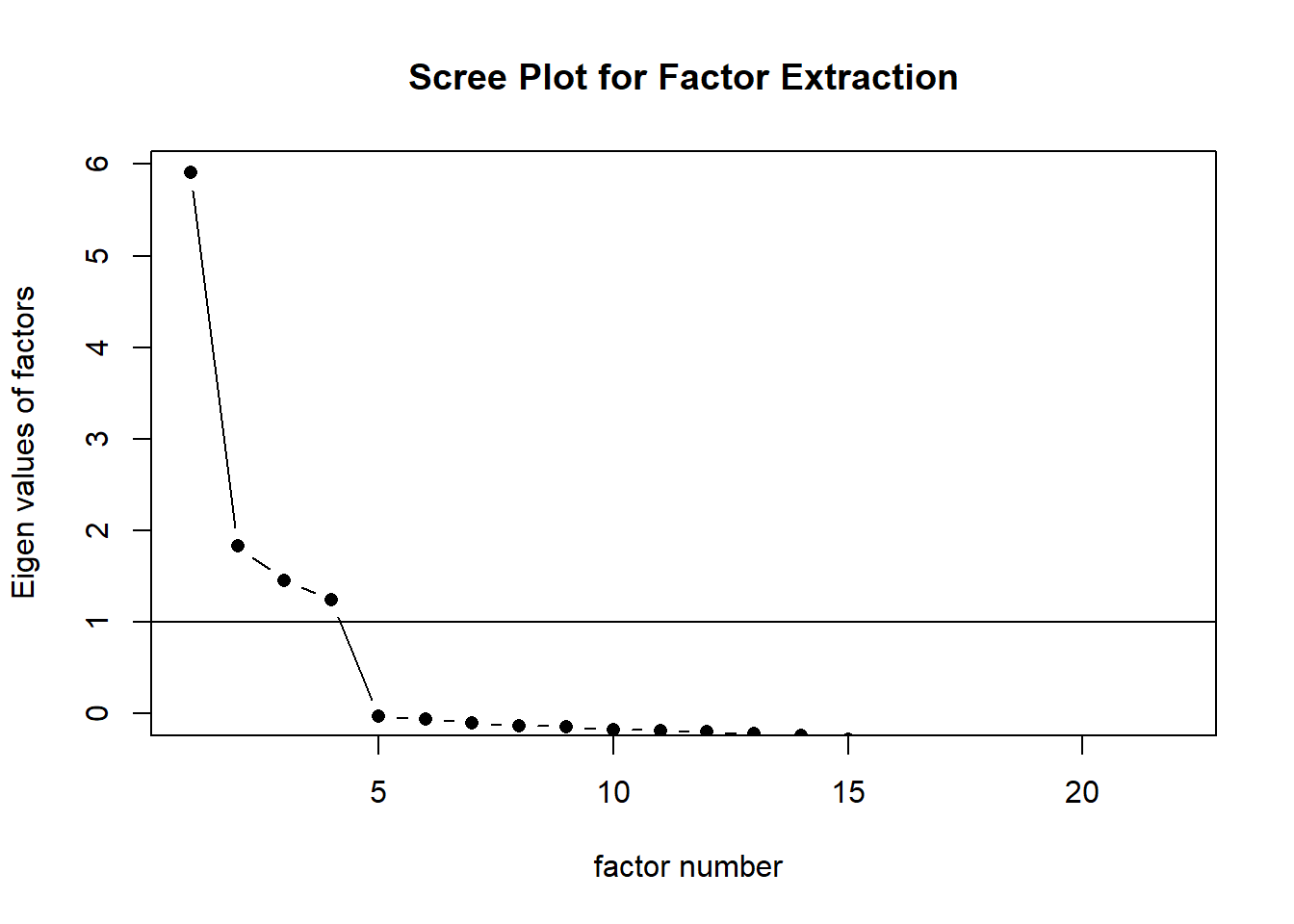
# 3. Parallel analysis
pa_result <- fa.parallel(scale_items, fm = "pa", fa = "fa", main = "Parallel Analysis")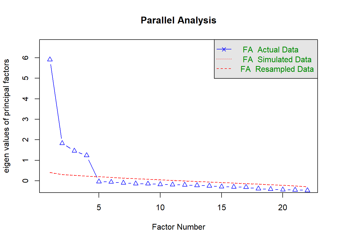
## Parallel analysis suggests that the number of factors = 4 and the number of components = NA## PARALLEL ANALYSIS:## Number of factors suggested: 4# 4. Very Simple Structure (VSS) complexity assessment
vss_result <- vss(scale_items, n = 8, rotate = "oblimin", diagonal = FALSE, fm = "pa")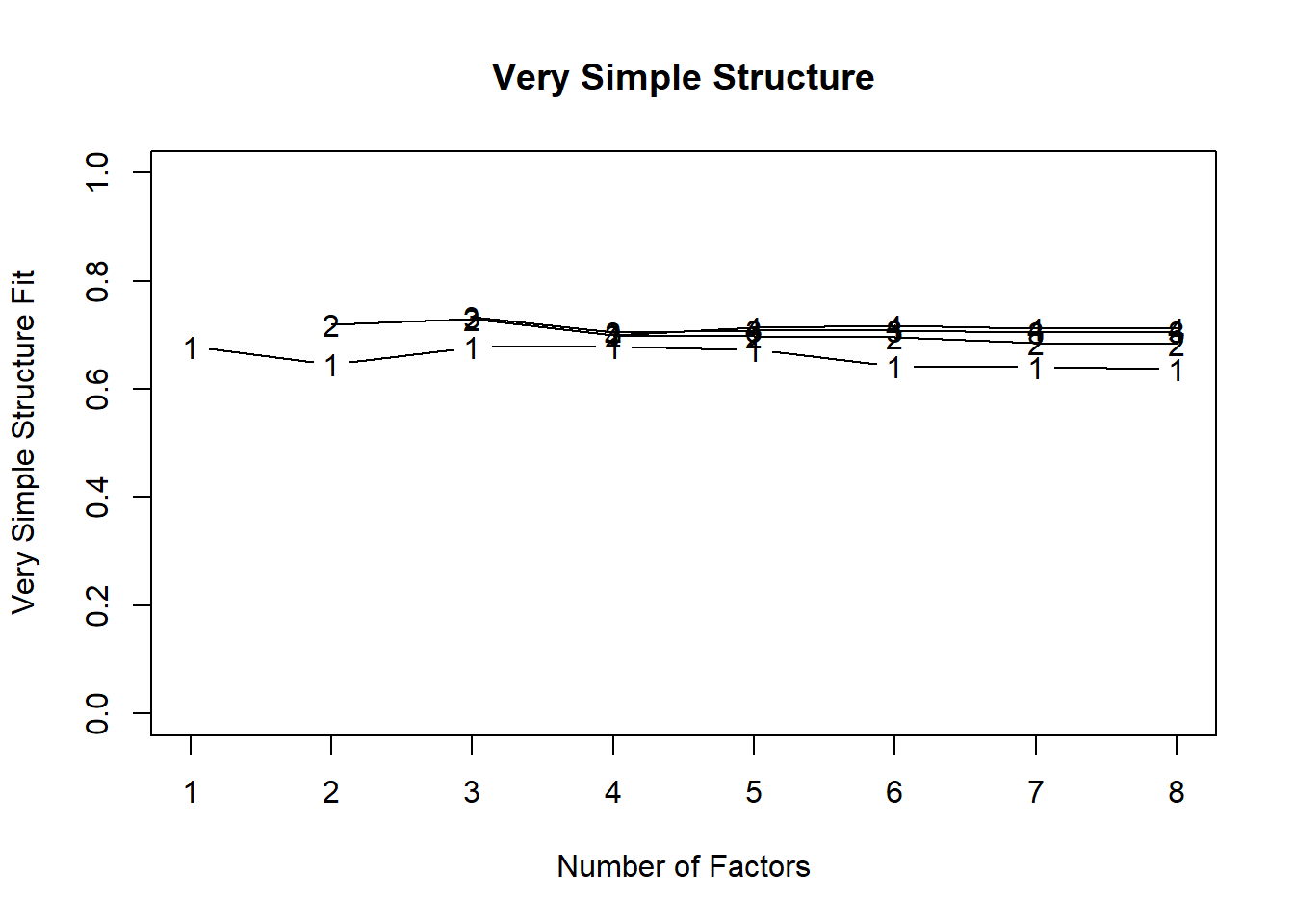
## VERY SIMPLE STRUCTURE (VSS) ANALYSIS:## Complexity 1 maximum at: 1 factors## Complexity 2 maximum at: 3 factors## FACTOR EXTRACTION SUMMARY:## Kaiser criterion: 4 factors## Parallel analysis: 4 factors## VSS complexity 1: 1 factors## VSS complexity 2: 3 factors## Theoretical expectation: 4 factors3.30.2 Conducting Exploratory Factor Analysis
Based on our factor extraction criteria and theoretical expectations, we’ll extract 4 factors and examine the solution.
3.30.2.1 EFA Decision Points:
- Extraction Method: Principal Axis Factoring (accounts for measurement error)
- Rotation Method: Oblique rotation (allows factors to correlate)
- Factor Loading Threshold: 0.40 for interpretation
- Cross-Loading Threshold: < 0.30 on non-primary factors
# Conduct EFA with 4 factors using Principal Axis Factoring and oblique rotation
efa_4factor <- fa(scale_items, nfactors = 4, rotate = "oblimin", fm = "pa",
                  max.iter = 100, scores = TRUE)

print(efa_4factor)
## Factor Analysis using method = pa
## Call: fa(r = scale_items, nfactors = 4, rotate = "oblimin", scores = TRUE,
## max.iter = 100, fm = "pa")
## Standardized loadings (pattern matrix) based upon correlation matrix
## PA1 PA4 PA2 PA3 h2 u2 com
## cog1 0.78 -0.01 0.00 0.01 0.60 0.40 1.0
## cog2 0.68 0.03 0.02 0.01 0.50 0.50 1.0
## cog3 0.82 -0.01 0.00 0.04 0.68 0.32 1.0
## cog4 0.61 -0.07 -0.03 -0.02 0.32 0.68 1.0
## cog5 0.74 0.08 -0.02 -0.04 0.58 0.42 1.0
## cog6 0.64 -0.02 0.06 0.03 0.44 0.56 1.0
## emo1 0.03 0.01 -0.02 0.82 0.68 0.32 1.0
## emo2 -0.02 -0.03 -0.02 0.82 0.64 0.36 1.0
## emo3 0.06 -0.04 0.05 0.63 0.42 0.58 1.0
## emo4 -0.01 0.06 0.03 0.73 0.57 0.43 1.0
## emo5 -0.01 0.03 0.00 0.57 0.33 0.67 1.0
## soc1 -0.01 0.00 0.78 0.00 0.60 0.40 1.0
## soc2 0.01 0.02 0.84 -0.02 0.72 0.28 1.0
## soc3 -0.05 0.03 0.63 0.04 0.41 0.59 1.0
## soc4 0.01 -0.01 0.78 0.03 0.62 0.38 1.0
## soc5 0.08 -0.04 0.60 -0.06 0.36 0.64 1.1
## beh1 0.01 0.74 0.02 0.00 0.57 0.43 1.0
## beh2 0.02 0.86 -0.03 -0.04 0.72 0.28 1.0
## beh3 -0.05 0.59 0.07 0.12 0.42 0.58 1.1
## beh4 0.01 0.72 0.00 0.04 0.55 0.45 1.0
## beh5 0.00 0.62 0.04 -0.05 0.39 0.61 1.0
## beh6 0.02 0.63 -0.03 0.02 0.40 0.60 1.0
##
## PA1 PA4 PA2 PA3
## SS loadings 3.13 3.02 2.74 2.66
## Proportion Var 0.14 0.14 0.12 0.12
## Cumulative Var 0.14 0.28 0.40 0.52
## Proportion Explained 0.27 0.26 0.24 0.23
## Cumulative Proportion 0.27 0.53 0.77 1.00
##
## With factor correlations of
## PA1 PA4 PA2 PA3
## PA1 1.00 0.49 0.30 0.38
## PA4 0.49 1.00 0.39 0.31
## PA2 0.30 0.39 1.00 0.21
## PA3 0.38 0.31 0.21 1.00
##
## Mean item complexity = 1
## Test of the hypothesis that 4 factors are sufficient.
##
## df null model = 231 with the objective function = 9.67 with Chi Square = 5714.43
## df of the model are 149 and the objective function was 0.27
##
## The root mean square of the residuals (RMSR) is 0.02
## The df corrected root mean square of the residuals is 0.02
##
## The harmonic n.obs is 600 with the empirical chi square 76.11 with prob < 1
## The total n.obs was 600 with Likelihood Chi Square = 158.32 with prob < 0.29
##
## Tucker Lewis Index of factoring reliability = 0.997
## RMSEA index = 0.01 and the 90 % confidence intervals are 0 0.022
## BIC = -794.83
## Fit based upon off diagonal values = 1
## Measures of factor score adequacy
## PA1 PA4 PA2 PA3
## Correlation of (regression) scores with factors 0.94 0.94 0.94 0.93
## Multiple R square of scores with factors 0.88 0.88 0.88 0.87
## Minimum correlation of possible factor scores 0.77 0.77 0.76 0.74##
## FACTOR LOADINGS INTERPRETATION:## Loading criteria: Primary loading > 0.40, Cross-loading < 0.30# Extract loadings matrix
loadings_matrix <- efa_4factor$loadings
class(loadings_matrix) <- "matrix"
# Identify items by factor based on highest loading
factor_assignment <- apply(abs(loadings_matrix), 1, which.max)
factor_labels <- c("Factor 1", "Factor 2", "Factor 3", "Factor 4")
for(i in 1:4) {
cat(factor_labels[i], "items:\n")
factor_items <- which(factor_assignment == i)
for(j in factor_items) {
primary_loading <- loadings_matrix[j, i]
cross_loadings <- loadings_matrix[j, -i]
max_cross <- max(abs(cross_loadings))
cat(" ", rownames(loadings_matrix)[j], ": primary =", round(primary_loading, 3),
", max cross =", round(max_cross, 3), "\n")
}
cat("\n")
}## Factor 1 items:
## cog1 : primary = 0.779 , max cross = 0.006
## cog2 : primary = 0.681 , max cross = 0.034
## cog3 : primary = 0.817 , max cross = 0.036
## cog4 : primary = 0.614 , max cross = 0.066
## cog5 : primary = 0.743 , max cross = 0.075
## cog6 : primary = 0.645 , max cross = 0.056
##
## Factor 2 items:
## beh1 : primary = 0.741 , max cross = 0.019
## beh2 : primary = 0.864 , max cross = 0.041
## beh3 : primary = 0.595 , max cross = 0.117
## beh4 : primary = 0.722 , max cross = 0.039
## beh5 : primary = 0.62 , max cross = 0.048
## beh6 : primary = 0.628 , max cross = 0.033
##
## Factor 3 items:
## soc1 : primary = 0.781 , max cross = 0.014
## soc2 : primary = 0.843 , max cross = 0.02
## soc3 : primary = 0.633 , max cross = 0.05
## soc4 : primary = 0.785 , max cross = 0.028
## soc5 : primary = 0.597 , max cross = 0.081
##
## Factor 4 items:
## emo1 : primary = 0.818 , max cross = 0.028
## emo2 : primary = 0.819 , max cross = 0.029
## emo3 : primary = 0.627 , max cross = 0.059
## emo4 : primary = 0.73 , max cross = 0.058
## emo5 : primary = 0.568 , max cross = 0.034## FACTOR CORRELATIONS:factor_cors <- efa_4factor$Phi
rownames(factor_cors) <- colnames(factor_cors) <- factor_labels
print(round(factor_cors, 3))## Factor 1 Factor 2 Factor 3 Factor 4
## Factor 1 1.000 0.491 0.300 0.380
## Factor 2 0.491 1.000 0.391 0.314
## Factor 3 0.300 0.391 1.000 0.210
## Factor 4 0.380 0.314 0.210 1.000##
## MODEL FIT ASSESSMENT:## Tucker Lewis Index (TLI): 0.997## Root Mean Square of Residuals (RMSR): 0.017cat("Chi-square test: χ² =", round(efa_4factor$STATISTIC, 2),
", df =", efa_4factor$dof, ", p =",
ifelse(efa_4factor$PVAL < 0.001, "< 0.001", round(efa_4factor$PVAL, 3)), "\n")## Chi-square test: χ² = 158.32 , df = 149 , p = 0.285# Proportion of variance explained
variance_explained <- efa_4factor$Vaccounted
cat("\nVARIANCE EXPLAINED:\n")##
## VARIANCE EXPLAINED:for(i in 1:4) {
cat("Factor", i, ": ", round(variance_explained[2, i] * 100, 1), "% of variance\n")
}## Factor 1 : 14.2 % of variance
## Factor 2 : 13.7 % of variance
## Factor 3 : 12.5 % of variance
## Factor 4 : 12.1 % of variance## Total variance explained: 52.5 %3.30.3 EFA Results Visualization
Visual representation helps interpret and communicate factor analysis results effectively.
# Create a comprehensive visualization of EFA results

# 1. Factor loading plot
par(mfrow = c(2, 2))

# Factor loading heatmap
loadings_for_plot <- loadings_matrix
colnames(loadings_for_plot) <- c("Cognitive", "Emotional", "Social", "Behavioral")

# Create color palette
colors <- colorRampPalette(c("darkred", "white", "darkblue"))(100)

# Plot heatmap
image(seq_len(ncol(loadings_for_plot)), seq_len(nrow(loadings_for_plot)),
      t(loadings_for_plot[rev(seq_len(nrow(loadings_for_plot))), ]),
      col = colors, axes = FALSE,
      main = "Factor Loadings Heatmap",
      xlab = "Factors", ylab = "Items")

# Add axes
axis(1, at = seq_len(ncol(loadings_for_plot)), labels = colnames(loadings_for_plot))
axis(2, at = seq_len(nrow(loadings_for_plot)),
     labels = rev(rownames(loadings_for_plot)), las = 2, cex.axis = 0.8)

# Add loading values as text
for(i in seq_len(nrow(loadings_for_plot))) {
  for(j in seq_len(ncol(loadings_for_plot))) {
    text(j, nrow(loadings_for_plot) - i + 1,
         round(loadings_for_plot[i, j], 2),
         col = ifelse(abs(loadings_for_plot[i, j]) > 0.5, "white", "black"),
         cex = 0.8)
  }
}

# 2. Scree plot
plot(eigenvalues[1:10], type = "b", pch = 19,
     main = "Scree Plot", xlab = "Factor Number", ylab = "Eigenvalue")
abline(h = 1, col = "red", lty = 2)
text(kaiser_factors + 0.5, 1.1, paste("Kaiser criterion:", kaiser_factors, "factors"),
     col = "red", cex = 0.8)

# 3. Factor correlation plot
factor_cors_plot <- factor_cors
diag(factor_cors_plot) <- NA
corrplot(factor_cors_plot, method = "color", type = "lower",
         diag = FALSE, title = "Factor Correlations",
         mar = c(0, 0, 2, 0), addCoef.col = "black")

# 4. Communalities plot
communalities <- efa_4factor$communality
barplot(sort(communalities, decreasing = TRUE),
        main = "Item Communalities",
        ylab = "Communality",
        las = 2, cex.names = 0.7)
abline(h = 0.3, col = "red", lty = 2)
text(length(communalities)/2, 0.35, "Minimum threshold (0.30)",
     col = "red", cex = 0.8)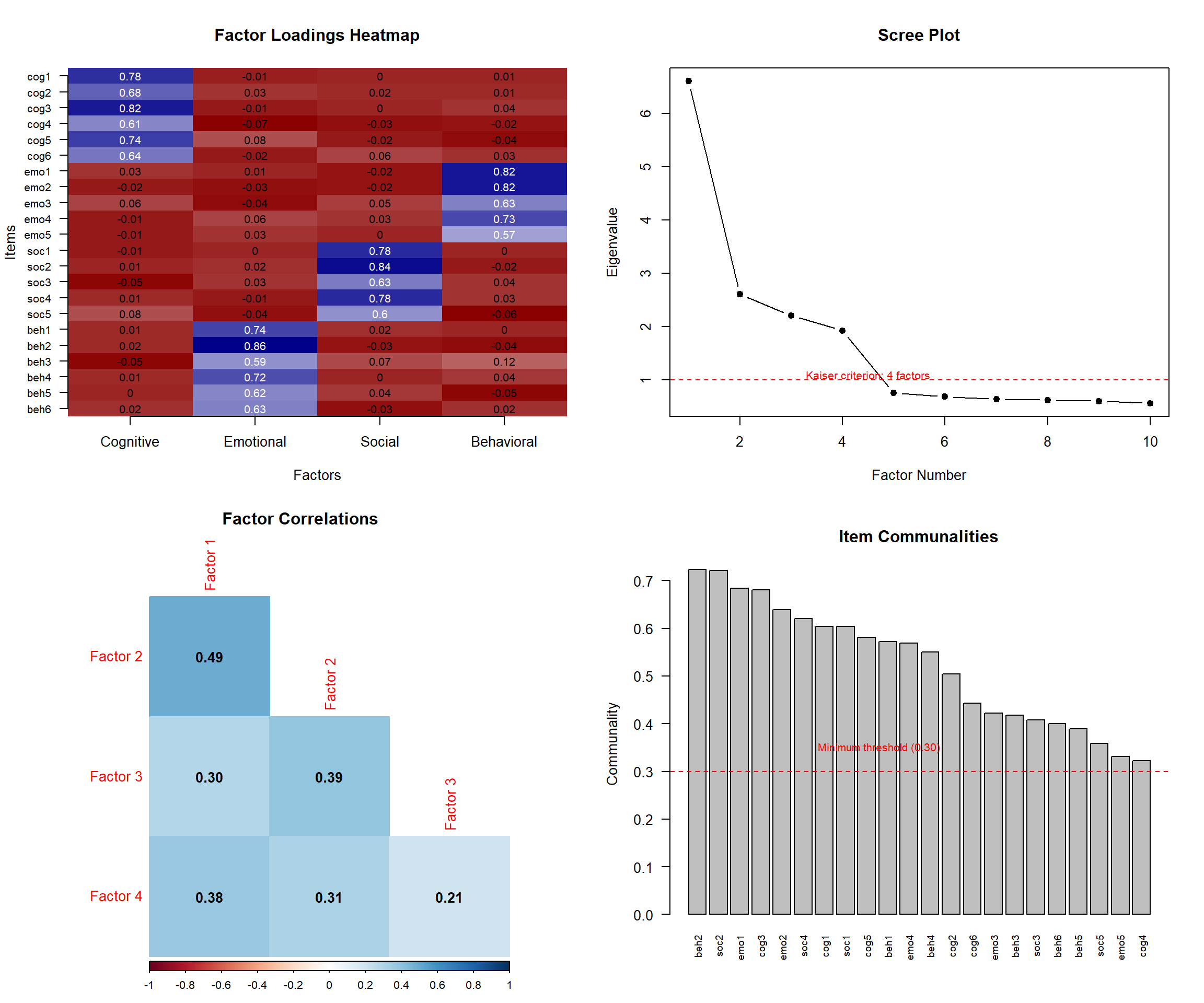
3.31 Confirmatory Factor Analysis (CFA)
3.31.1 Testing the EFA-Derived Model
Now we’ll use CFA to test the factor structure identified in our EFA. This provides a more rigorous test of our proposed model.
3.31.1.1 CFA Model Specification:
Based on EFA results, we’ll specify a 4-factor model with items loading on their respective factors and allowing factors to correlate.
# Specify CFA model based on EFA results
# Note: In practice, you might use a separate sample for CFA

cfa_model <- '
  # Cognitive Resilience
  cognitive =~ cog1 + cog2 + cog3 + cog4 + cog5 + cog6

  # Emotional Resilience
  emotional =~ emo1 + emo2 + emo3 + emo4 + emo5

  # Social Resilience
  social =~ soc1 + soc2 + soc3 + soc4 + soc5

  # Behavioral Resilience
  behavioral =~ beh1 + beh2 + beh3 + beh4 + beh5 + beh6
'

# Fit the CFA model
cfa_fit <- cfa(cfa_model, data = scale_items, estimator = "MLR")

# Model summary
summary(cfa_fit, fit.measures = TRUE, standardized = TRUE)
## lavaan 0.6-19 ended normally after 35 iterations
##
## Estimator ML
## Optimization method NLMINB
## Number of model parameters 50
##
## Number of observations 600
##
## Model Test User Model:
## Standard Scaled
## Test Statistic 219.401 219.461
## Degrees of freedom 203 203
## P-value (Chi-square) 0.204 0.204
## Scaling correction factor 1.000
## Yuan-Bentler correction (Mplus variant)
##
## Model Test Baseline Model:
##
## Test statistic 5803.086 5776.267
## Degrees of freedom 231 231
## P-value 0.000 0.000
## Scaling correction factor 1.005
##
## User Model versus Baseline Model:
##
## Comparative Fit Index (CFI) 0.997 0.997
## Tucker-Lewis Index (TLI) 0.997 0.997
##
## Robust Comparative Fit Index (CFI) 0.997
## Robust Tucker-Lewis Index (TLI) 0.997
##
## Loglikelihood and Information Criteria:
##
## Loglikelihood user model (H0) -16368.500 -16368.500
## Scaling correction factor 1.002
## for the MLR correction
## Loglikelihood unrestricted model (H1) -16258.799 -16258.799
## Scaling correction factor 1.000
## for the MLR correction
##
## Akaike (AIC) 32836.999 32836.999
## Bayesian (BIC) 33056.846 33056.846
## Sample-size adjusted Bayesian (SABIC) 32898.110 32898.110
##
## Root Mean Square Error of Approximation:
##
## RMSEA 0.012 0.012
## 90 Percent confidence interval - lower 0.000 0.000
## 90 Percent confidence interval - upper 0.022 0.022
## P-value H_0: RMSEA <= 0.050 1.000 1.000
## P-value H_0: RMSEA >= 0.080 0.000 0.000
##
## Robust RMSEA 0.012
## 90 Percent confidence interval - lower 0.000
## 90 Percent confidence interval - upper 0.022
## P-value H_0: Robust RMSEA <= 0.050 1.000
## P-value H_0: Robust RMSEA >= 0.080 0.000
##
## Standardized Root Mean Square Residual:
##
## SRMR 0.029 0.029
##
## Parameter Estimates:
##
## Standard errors Sandwich
## Information bread Observed
## Observed information based on Hessian
##
## Latent Variables:
## Estimate Std.Err z-value P(>|z|) Std.lv Std.all
## cognitive =~
## cog1 1.000 0.802 0.776
## cog2 0.867 0.046 18.916 0.000 0.695 0.712
## cog3 1.074 0.054 19.863 0.000 0.861 0.825
## cog4 0.723 0.059 12.315 0.000 0.579 0.551
## cog5 0.974 0.050 19.448 0.000 0.781 0.765
## cog6 0.840 0.052 16.179 0.000 0.673 0.662
## emotional =~
## emo1 1.000 0.869 0.829
## emo2 0.956 0.045 21.160 0.000 0.831 0.784
## emo3 0.795 0.046 17.341 0.000 0.691 0.655
## emo4 0.848 0.043 19.744 0.000 0.737 0.755
## emo5 0.683 0.049 13.969 0.000 0.593 0.572
## social =~
## soc1 1.000 0.842 0.775
## soc2 1.094 0.050 21.968 0.000 0.922 0.849
## soc3 0.782 0.050 15.650 0.000 0.659 0.646
## soc4 0.928 0.046 20.042 0.000 0.782 0.780
## soc5 0.739 0.053 13.920 0.000 0.623 0.595
## behavioral =~
## beh1 1.000 0.786 0.763
## beh2 1.093 0.053 20.717 0.000 0.859 0.842
## beh3 0.851 0.053 16.012 0.000 0.669 0.639
## beh4 0.961 0.051 18.780 0.000 0.755 0.742
## beh5 0.840 0.057 14.640 0.000 0.660 0.619
## beh6 0.797 0.056 14.305 0.000 0.627 0.630
##
## Covariances:
## Estimate Std.Err z-value P(>|z|) Std.lv Std.all
## cognitive ~~
## emotional 0.279 0.038 7.381 0.000 0.401 0.401
## social 0.211 0.033 6.363 0.000 0.312 0.312
## behavioral 0.320 0.034 9.524 0.000 0.507 0.507
## emotional ~~
## social 0.158 0.035 4.467 0.000 0.216 0.216
## behavioral 0.229 0.037 6.269 0.000 0.335 0.335
## social ~~
## behavioral 0.267 0.034 7.869 0.000 0.403 0.403
##
## Variances:
## Estimate Std.Err z-value P(>|z|) Std.lv Std.all
## .cog1 0.425 0.035 12.224 0.000 0.425 0.398
## .cog2 0.471 0.031 14.983 0.000 0.471 0.493
## .cog3 0.349 0.030 11.516 0.000 0.349 0.320
## .cog4 0.770 0.044 17.442 0.000 0.770 0.696
## .cog5 0.431 0.030 14.479 0.000 0.431 0.414
## .cog6 0.580 0.037 15.754 0.000 0.580 0.561
## .emo1 0.344 0.032 10.681 0.000 0.344 0.313
## .emo2 0.432 0.034 12.695 0.000 0.432 0.385
## .emo3 0.635 0.040 15.726 0.000 0.635 0.571
## .emo4 0.409 0.031 13.190 0.000 0.409 0.430
## .emo5 0.725 0.045 16.280 0.000 0.725 0.673
## .soc1 0.472 0.033 14.266 0.000 0.472 0.400
## .soc2 0.329 0.030 10.826 0.000 0.329 0.279
## .soc3 0.606 0.038 16.093 0.000 0.606 0.583
## .soc4 0.394 0.033 11.827 0.000 0.394 0.392
## .soc5 0.708 0.042 16.776 0.000 0.708 0.646
## .beh1 0.444 0.033 13.371 0.000 0.444 0.418
## .beh2 0.304 0.027 11.178 0.000 0.304 0.291
## .beh3 0.650 0.044 14.919 0.000 0.650 0.592
## .beh4 0.464 0.032 14.595 0.000 0.464 0.449
## .beh5 0.704 0.043 16.191 0.000 0.704 0.617
## .beh6 0.595 0.038 15.588 0.000 0.595 0.603
## cognitive 0.643 0.058 11.099 0.000 1.000 1.000
## emotional 0.755 0.062 12.273 0.000 1.000 1.000
## social 0.710 0.065 10.914 0.000 1.000 1.000
## behavioral 0.618 0.057 10.800 0.000 1.000 1.000# Extract fit measures for reporting
fit_measures <- fitMeasures(cfa_fit, c("chisq", "df", "pvalue", "cfi", "tli",
"rmsea", "rmsea.ci.lower", "rmsea.ci.upper",
"srmr", "aic", "bic"))
cat("\nCFA MODEL FIT SUMMARY:\n")##
## CFA MODEL FIT SUMMARY:cat("χ² =", round(fit_measures["chisq"], 2), ", df =", fit_measures["df"],
", p =", ifelse(fit_measures["pvalue"] < 0.001, "< 0.001", round(fit_measures["pvalue"], 3)), "\n")## χ² = 219.4 , df = 203 , p = 0.204## CFI = 0.997 (> 0.95 excellent, > 0.90 acceptable)## TLI = 0.997 (> 0.95 excellent, > 0.90 acceptable)## RMSEA = 0.012 (< 0.06 excellent, < 0.08 acceptable)cat("RMSEA 90% CI: [", round(fit_measures["rmsea.ci.lower"], 3), ", ",
round(fit_measures["rmsea.ci.upper"], 3), "]\n")## RMSEA 90% CI: [ 0 , 0.022 ]## SRMR = 0.029 (< 0.08 acceptable)##
## STANDARDIZED FACTOR LOADINGS:loadings_cfa <- standardizedSolution(cfa_fit)
factor_loadings <- loadings_cfa[loadings_cfa$op == "=~", ]
print(factor_loadings[, c("lhs", "rhs", "est.std", "pvalue")])## lhs rhs est.std pvalue
## 1 cognitive cog1 0.776 0
## 2 cognitive cog2 0.712 0
## 3 cognitive cog3 0.825 0
## 4 cognitive cog4 0.551 0
## 5 cognitive cog5 0.765 0
## 6 cognitive cog6 0.662 0
## 7 emotional emo1 0.829 0
## 8 emotional emo2 0.784 0
## 9 emotional emo3 0.655 0
## 10 emotional emo4 0.755 0
## 11 emotional emo5 0.572 0
## 12 social soc1 0.775 0
## 13 social soc2 0.849 0
## 14 social soc3 0.646 0
## 15 social soc4 0.780 0
## 16 social soc5 0.595 0
## 17 behavioral beh1 0.763 0
## 18 behavioral beh2 0.842 0
## 19 behavioral beh3 0.639 0
## 20 behavioral beh4 0.742 0
## 21 behavioral beh5 0.619 0
## 22 behavioral beh6 0.630 0##
## FACTOR CORRELATIONS:factor_corrs_cfa <- loadings_cfa[loadings_cfa$op == "~~" & loadings_cfa$lhs != loadings_cfa$rhs, ]
if(nrow(factor_corrs_cfa) > 0) {
print(factor_corrs_cfa[, c("lhs", "rhs", "est.std", "pvalue")])
}## lhs rhs est.std pvalue
## 49 cognitive emotional 0.401 0
## 50 cognitive social 0.312 0
## 51 cognitive behavioral 0.507 0
## 52 emotional social 0.216 0
## 53 emotional behavioral 0.335 0
## 54 social behavioral 0.403 03.31.2 CFA Model Diagnostics and Improvement
If the initial model fit is not acceptable, we examine modification indices and residuals to identify potential improvements.
# Modification indices
mod_indices <- modificationIndices(cfa_fit, sort = TRUE, maximum.number = 10)
cat("TOP 10 MODIFICATION INDICES:\n")
## TOP 10 MODIFICATION INDICES:## lhs op rhs mi epc
## 190 cog4 ~~ soc3 10.531 -0.097
## 84 emotional =~ beh3 9.093 0.140
## 133 cog1 ~~ soc3 6.750 0.062
## 324 soc4 ~~ soc5 6.278 0.067
## 328 soc4 ~~ beh4 6.247 -0.053
## 134 cog1 ~~ soc4 6.073 -0.050
## 261 emo3 ~~ emo4 5.564 -0.063
## 317 soc3 ~~ soc5 5.276 -0.069
## 307 soc2 ~~ soc3 5.025 0.062
## 329 soc4 ~~ beh5 4.802 0.054# Residual correlations
residuals_cfa <- residuals(cfa_fit, type = "cor")
cat("\nLARGEST RESIDUAL CORRELATIONS (absolute value > 0.10):\n")##
## LARGEST RESIDUAL CORRELATIONS (absolute value > 0.10):# Check if residuals were successfully extracted
if(!is.null(residuals_cfa) && is.matrix(residuals_cfa)) {
residual_matrix <- residuals_cfa
residual_matrix[upper.tri(residual_matrix, diag = TRUE)] <- NA
large_residuals <- which(abs(residual_matrix) > 0.10, arr.ind = TRUE)
if(nrow(large_residuals) > 0) {
for(i in seq_len(nrow(large_residuals))) {
row_name <- rownames(residual_matrix)[large_residuals[i, 1]]
col_name <- colnames(residual_matrix)[large_residuals[i, 2]]
residual_value <- residual_matrix[large_residuals[i, 1], large_residuals[i, 2]]
cat(row_name, "-", col_name, ":", round(residual_value, 3), "\n")
}
} else {
cat("No large residual correlations detected\n")
}
} else {
# Alternative approach: examine modification indices for problematic residuals
cat("Residual matrix not available; examining modification indices instead\n")
high_mi <- mod_indices[mod_indices$mi > 10, ]
if(nrow(high_mi) > 0) {
cat("High modification indices (> 10) suggesting model misspecification:\n")
print(high_mi[, c("lhs", "op", "rhs", "mi")])
} else {
cat("No major model misspecifications detected\n")
}
}## Residual matrix not available; examining modification indices instead
## High modification indices (> 10) suggesting model misspecification:
## lhs op rhs mi
## 190 cog4 ~~ soc3 10.531# Local fit assessment
local_fit <- inspect(cfa_fit, "r2")
cat("\nR-SQUARED VALUES (proportion of variance explained):\n")##
## R-SQUARED VALUES (proportion of variance explained):## cog1 cog2 cog3 cog4 cog5 cog6 emo1 emo2 emo3 emo4 emo5 soc1 soc2
## 0.602 0.507 0.680 0.304 0.586 0.439 0.687 0.615 0.429 0.570 0.327 0.600 0.721
## soc3 soc4 soc5 beh1 beh2 beh3 beh4 beh5 beh6
## 0.417 0.608 0.354 0.582 0.709 0.408 0.551 0.383 0.397# Check for problematic items (low loadings or poor fit)
low_loadings <- factor_loadings[factor_loadings$est.std < 0.50, ]
cat("\nITEMS WITH LOW LOADINGS (< 0.50):\n")##
## ITEMS WITH LOW LOADINGS (< 0.50):if(nrow(low_loadings) > 0) {
print(low_loadings[, c("rhs", "est.std")])
} else {
cat("No items with low loadings\n")
}## No items with low loadings3.31.3 CFA Visualization
# Create path diagram of CFA model
semPaths(cfa_fit, what = "std", whatLabels = "std",
         style = "lisrel", layout = "tree2", rotation = 2,
         sizeLat = 8, sizeMan = 4, edge.label.cex = 0.8,
         title = FALSE, curvePivot = TRUE)
title("Confirmatory Factor Analysis: Academic Resilience Scale")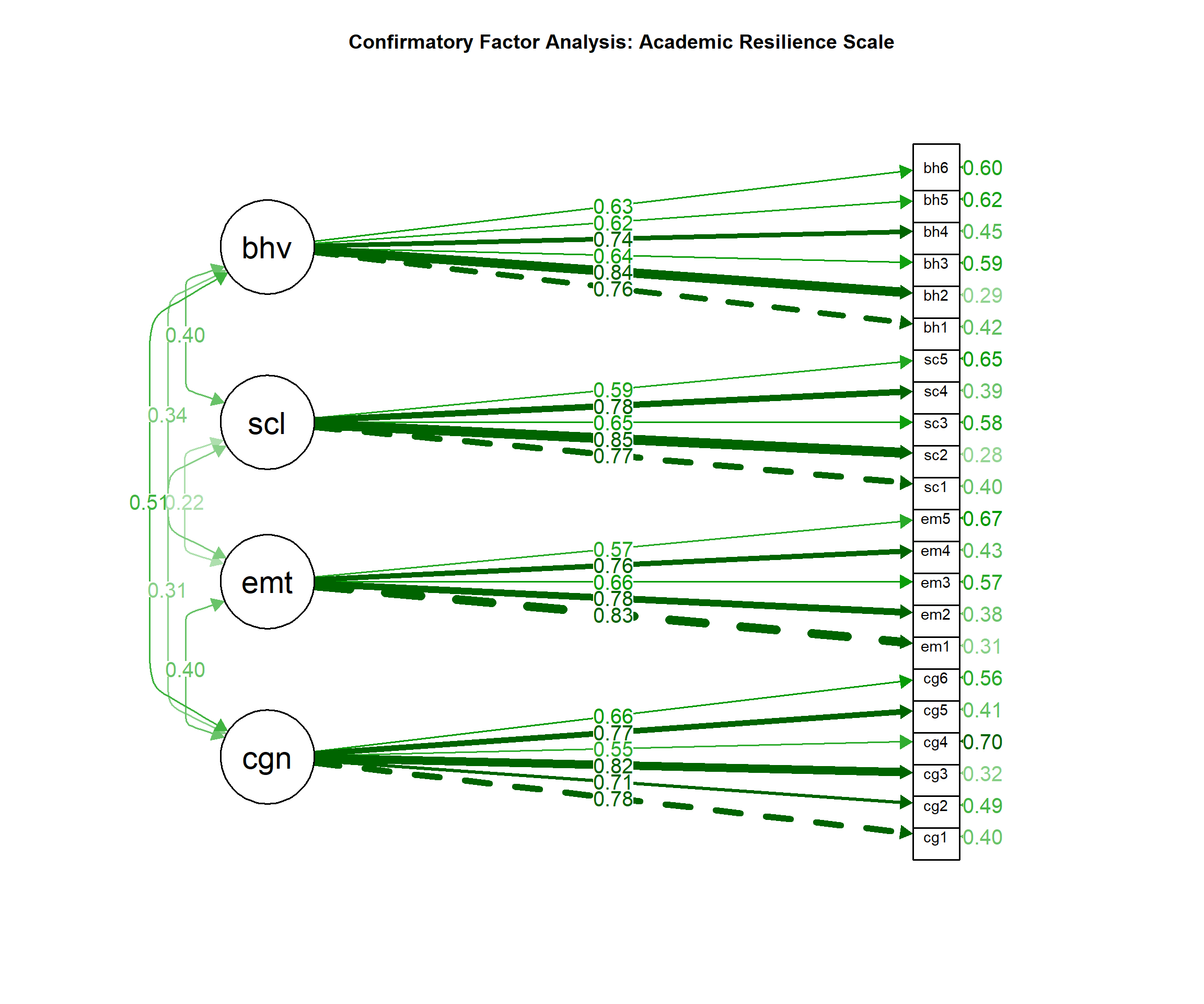
# Alternative diagram with factor correlations emphasized
semPaths(cfa_fit, what = "std", whatLabels = "std",
         style = "lisrel", layout = "circle", rotation = 1,
         sizeLat = 10, sizeMan = 3, edge.label.cex = 0.7,
         title = FALSE, curve = 2)
title("CFA Model: Correlated Four-Factor Structure")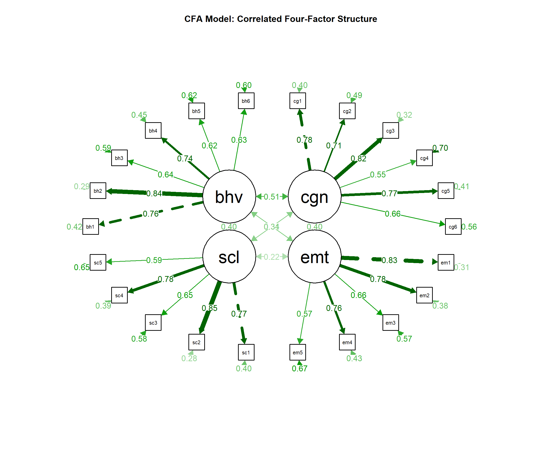
3.32 Reliability and Internal Consistency
3.32.1 Multiple Reliability Indices
We’ll calculate several reliability indices to assess the internal consistency of our factors.
# Calculate reliability for each factor using multiple methods

# Extract items for each factor based on CFA loadings
cognitive_items <- scale_items[, c("cog1", "cog2", "cog3", "cog4", "cog5", "cog6")]
emotional_items <- scale_items[, c("emo1", "emo2", "emo3", "emo4", "emo5")]
social_items <- scale_items[, c("soc1", "soc2", "soc3", "soc4", "soc5")]
behavioral_items <- scale_items[, c("beh1", "beh2", "beh3", "beh4", "beh5", "beh6")]

# Function to calculate comprehensive reliability statistics
calculate_reliability <- function(items, factor_name) {
  cat("\n", toupper(factor_name), "RELIABILITY:\n")
  cat("Number of items:", ncol(items), "\n")

  # Cronbach's alpha
  alpha_result <- psych::alpha(items)
  cat("Cronbach's α =", round(alpha_result$total$std.alpha, 3), "\n")

  # Omega coefficients
  omega_result <- psych::omega(items, nfactors = 1, plot = FALSE)
  cat("McDonald's ω =", round(omega_result$omega.tot, 3), "\n")
  cat("ω hierarchical =", round(omega_result$omega_h, 3), "\n")

  # Item-total correlations
  cat("Item-total correlations:\n")
  item_total_cors <- alpha_result$item.stats$r.cor
  for(i in seq_along(item_total_cors)) {
    cat(" ", names(item_total_cors)[i], ":", round(item_total_cors[i], 3), "\n")
  }

  # Alpha if item deleted
  cat("α if item deleted:\n")
  alpha_if_deleted <- alpha_result$alpha.drop$std.alpha
  for(i in seq_along(alpha_if_deleted)) {
    cat(" ", names(alpha_if_deleted)[i], ":", round(alpha_if_deleted[i], 3), "\n")
  }

  return(list(alpha = alpha_result$total$std.alpha,
              omega = omega_result$omega.tot,
              omega_h = omega_result$omega_h))
}

# Calculate reliability for each factor
cognitive_rel <- calculate_reliability(cognitive_items, "Cognitive Resilience")
##
## COGNITIVE RESILIENCE RELIABILITY:
## Number of items: 6
## Cronbach's α = 0.862## McDonald's ω = 0.865
## ω hierarchical = 0.865
## Item-total correlations:
## : 0.767
## : 0.703
## : 0.811
## : 0.555
## : 0.75
## : 0.656
## α if item deleted:
## : 0.829
## : 0.839
## : 0.821
## : 0.863
## : 0.832
## : 0.847##
## EMOTIONAL RESILIENCE RELIABILITY:
## Number of items: 5
## Cronbach's α = 0.841## McDonald's ω = 0.845
## ω hierarchical = 0.845
## Item-total correlations:
## : 0.805
## : 0.776
## : 0.645
## : 0.736
## : 0.571
## α if item deleted:
## : 0.784
## : 0.791
## : 0.824
## : 0.802
## : 0.84##
## SOCIAL RESILIENCE RELIABILITY:
## Number of items: 5
## Cronbach's α = 0.848## McDonald's ω = 0.852
## ω hierarchical = 0.852
## Item-total correlations:
## : 0.764
## : 0.827
## : 0.632
## : 0.773
## : 0.589
## α if item deleted:
## : 0.805
## : 0.789
## : 0.838
## : 0.803
## : 0.847##
## BEHAVIORAL RESILIENCE RELIABILITY:
## Number of items: 6
## Cronbach's α = 0.855## McDonald's ω = 0.857
## ω hierarchical = 0.857
## Item-total correlations:
## : 0.747
## : 0.829
## : 0.626
## : 0.732
## : 0.616
## : 0.628
## α if item deleted:
## : 0.822
## : 0.807
## : 0.842
## : 0.825
## : 0.844
## : 0.842# Summary table
reliability_summary <- data.frame(
Factor = c("Cognitive", "Emotional", "Social", "Behavioral"),
Items = c(6, 5, 5, 6),
Alpha = c(cognitive_rel$alpha, emotional_rel$alpha,
social_rel$alpha, behavioral_rel$alpha),
Omega = c(cognitive_rel$omega, emotional_rel$omega,
social_rel$omega, behavioral_rel$omega),
Omega_h = c(cognitive_rel$omega_h, emotional_rel$omega_h,
social_rel$omega_h, behavioral_rel$omega_h)
)
cat("\n\nRELIABILITY SUMMARY TABLE:\n")##
##
## RELIABILITY SUMMARY TABLE:# Round only the numeric columns
reliability_summary_rounded <- reliability_summary
reliability_summary_rounded[, c("Alpha", "Omega", "Omega_h")] <- round(reliability_summary_rounded[, c("Alpha", "Omega", "Omega_h")], 3)
print(reliability_summary_rounded)## Factor Items Alpha Omega Omega_h
## 1 Cognitive 6 0.862 0.865 0.865
## 2 Emotional 5 0.841 0.845 0.845
## 3 Social 5 0.848 0.852 0.852
## 4 Behavioral 6 0.855 0.857 0.857##
## INTERPRETATION GUIDELINES:## α/ω ≥ 0.90: Excellent reliability## α/ω ≥ 0.80: Good reliability## α/ω ≥ 0.70: Acceptable reliability## α/ω < 0.70: Poor reliability3.33 Validity Evidence
3.33.1 Convergent and Discriminant Validity
We’ll examine evidence for construct validity using the CFA results.
# Extract standardized loadings and construct reliability/variance extracted measures
std_loadings <- standardizedSolution(cfa_fit)
factor_loadings_only <- std_loadings[std_loadings$op == "=~", ]

# Calculate Average Variance Extracted (AVE) and Composite Reliability (CR)
calculate_ave_cr <- function(loadings) {
  loadings_sq <- loadings^2
  ave <- sum(loadings_sq) / (sum(loadings_sq) + sum(1 - loadings_sq))
  cr <- (sum(loadings))^2 / ((sum(loadings))^2 + sum(1 - loadings_sq))
  return(list(ave = ave, cr = cr))
}

# Calculate for each factor
cognitive_loadings <- factor_loadings_only[factor_loadings_only$lhs == "cognitive", "est.std"]
emotional_loadings <- factor_loadings_only[factor_loadings_only$lhs == "emotional", "est.std"]
social_loadings <- factor_loadings_only[factor_loadings_only$lhs == "social", "est.std"]
behavioral_loadings <- factor_loadings_only[factor_loadings_only$lhs == "behavioral", "est.std"]

cognitive_validity <- calculate_ave_cr(cognitive_loadings)
emotional_validity <- calculate_ave_cr(emotional_loadings)
social_validity <- calculate_ave_cr(social_loadings)
behavioral_validity <- calculate_ave_cr(behavioral_loadings)

# Validity summary
validity_summary <- data.frame(
  Factor = c("Cognitive", "Emotional", "Social", "Behavioral"),
  CR = c(cognitive_validity$cr, emotional_validity$cr,
         social_validity$cr, behavioral_validity$cr),
  AVE = c(cognitive_validity$ave, emotional_validity$ave,
          social_validity$ave, behavioral_validity$ave),
  AVE_sqrt = sqrt(c(cognitive_validity$ave, emotional_validity$ave,
                    social_validity$ave, behavioral_validity$ave))
)

cat("CONSTRUCT VALIDITY EVIDENCE:\n\n")
## CONSTRUCT VALIDITY EVIDENCE:# Round only numeric columns
validity_summary_rounded <- validity_summary
validity_summary_rounded[sapply(validity_summary_rounded, is.numeric)] <-
round(validity_summary_rounded[sapply(validity_summary_rounded, is.numeric)], 3)
print(validity_summary_rounded)## Factor CR AVE AVE_sqrt
## 1 Cognitive 0.865 0.520 0.721
## 2 Emotional 0.845 0.526 0.725
## 3 Social 0.852 0.540 0.735
## 4 Behavioral 0.858 0.505 0.711##
## CONVERGENT VALIDITY:## Composite Reliability (CR) > 0.70: Good convergent validity## Average Variance Extracted (AVE) > 0.50: Adequate convergent validity# Factor correlations for discriminant validity assessment
factor_cors_validity <- std_loadings[std_loadings$op == "~~" &
std_loadings$lhs != std_loadings$rhs, ]
cat("DISCRIMINANT VALIDITY:\n")## DISCRIMINANT VALIDITY:## Factor correlations should be < √AVE for each factorif(nrow(factor_cors_validity) > 0) {
cat("Factor correlations:\n")
for(i in seq_len(nrow(factor_cors_validity))) {
cat(factor_cors_validity$lhs[i], "-", factor_cors_validity$rhs[i], ":",
round(factor_cors_validity$est.std[i], 3), "\n")
}
cat("\nDiscriminant validity assessment:\n")
max_correlation <- max(abs(factor_cors_validity$est.std))
min_ave_sqrt <- min(validity_summary$AVE_sqrt)
cat("Highest factor correlation:", round(max_correlation, 3), "\n")
cat("Lowest √AVE:", round(min_ave_sqrt, 3), "\n")
if(max_correlation < min_ave_sqrt) {
cat("✓ Discriminant validity supported\n")
} else {
cat("✗ Discriminant validity questionable\n")
}
}## Factor correlations:
## cognitive - emotional : 0.401
## cognitive - social : 0.312
## cognitive - behavioral : 0.507
## emotional - social : 0.216
## emotional - behavioral : 0.335
## social - behavioral : 0.403
##
## Discriminant validity assessment:
## Highest factor correlation: 0.507
## Lowest √AVE: 0.711
## ✓ Discriminant validity supported3.34 Scale Scoring and Final Recommendations
3.34.1 Creating Factor Scores
We’ll create factor scores for practical use of the scale.
# Calculate factor scores using different methods

# 1. Simple sum scores (unit-weighted)
cognitive_sum <- rowSums(cognitive_items)
emotional_sum <- rowSums(emotional_items)
social_sum <- rowSums(social_items)
behavioral_sum <- rowSums(behavioral_items)

# 2. Mean scores (for easier interpretation)
cognitive_mean <- rowMeans(cognitive_items)
emotional_mean <- rowMeans(emotional_items)
social_mean <- rowMeans(social_items)
behavioral_mean <- rowMeans(behavioral_items)

# 3. Factor scores from CFA (regression method)
factor_scores <- lavPredict(cfa_fit)

# Create final dataset with scores
final_scores <- data.frame(
  # Demographics
  age = resilience_data$age,
  gender = resilience_data$gender,
  year_in_school = resilience_data$year_in_school,
  gpa = resilience_data$gpa,

  # Sum scores
  cognitive_sum = cognitive_sum,
  emotional_sum = emotional_sum,
  social_sum = social_sum,
  behavioral_sum = behavioral_sum,

  # Mean scores
  cognitive_mean = cognitive_mean,
  emotional_mean = emotional_mean,
  social_mean = social_mean,
  behavioral_mean = behavioral_mean,

  # Factor scores
  cognitive_factor = factor_scores[, "cognitive"],
  emotional_factor = factor_scores[, "emotional"],
  social_factor = factor_scores[, "social"],
  behavioral_factor = factor_scores[, "behavioral"]
)

# Descriptive statistics for scores
cat("SCALE SCORE DESCRIPTIVES:\n\n")
## SCALE SCORE DESCRIPTIVES:## Sum Scores (possible range: 5-35 for 5-item scales, 6-42 for 6-item scales):## vars n mean sd median trimmed mad min max range skew
## cognitive_sum 1 600 24.48 4.73 25 24.53 4.45 9 38 29 -0.09
## emotional_sum 2 600 20.31 4.05 20 20.30 4.45 8 34 26 -0.01
## social_sum 3 600 20.25 4.14 20 20.21 4.45 8 35 27 0.10
## behavioral_sum 4 600 24.16 4.71 24 24.24 4.45 9 38 29 -0.15
## kurtosis se
## cognitive_sum -0.23 0.19
## emotional_sum -0.04 0.17
## social_sum 0.10 0.17
## behavioral_sum -0.04 0.19##
## Mean Scores (possible range: 1-7):## vars n mean sd median trimmed mad min max range skew
## cognitive_mean 1 600 4.08 0.79 4.17 4.09 0.74 1.5 6.33 4.83 -0.09
## emotional_mean 2 600 4.06 0.81 4.00 4.06 0.89 1.6 6.80 5.20 -0.01
## social_mean 3 600 4.05 0.83 4.00 4.04 0.89 1.6 7.00 5.40 0.10
## behavioral_mean 4 600 4.03 0.78 4.00 4.04 0.74 1.5 6.33 4.83 -0.15
## kurtosis se
## cognitive_mean -0.23 0.03
## emotional_mean -0.04 0.03
## social_mean 0.10 0.03
## behavioral_mean -0.04 0.03# Correlations between scoring methods
score_correlations <- cor(final_scores[, 5:16])
cat("\nCORRELATIONS BETWEEN SCORING METHODS:\n")##
## CORRELATIONS BETWEEN SCORING METHODS:## Sum vs Mean scores should be r = 1.00## Sum/Mean vs Factor scores should be high (r > 0.90)# Show correlations for cognitive factor as example
cog_cors <- score_correlations[c("cognitive_sum", "cognitive_mean", "cognitive_factor"),
c("cognitive_sum", "cognitive_mean", "cognitive_factor")]
print(round(cog_cors, 3))## cognitive_sum cognitive_mean cognitive_factor
## cognitive_sum 1.000 1.000 0.988
## cognitive_mean 1.000 1.000 0.988
## cognitive_factor 0.988 0.988 1.0003.34.2 Scale Administration Guidelines
## ACADEMIC RESILIENCE INVENTORY (ARI) ADMINISTRATION GUIDELINES:## SCALE DESCRIPTION:## The ARI is a 22-item measure assessing four dimensions of academic resilience:## - Cognitive Resilience (6 items): Positive thinking and problem-solving## - Emotional Resilience (5 items): Emotional regulation during academic stress## - Social Resilience (5 items): Help-seeking and social support utilization## - Behavioral Resilience (6 items): Persistence and adaptive strategies## RESPONSE FORMAT:## 7-point Likert scale: 1 = Strongly Disagree, 7 = Strongly Agree## All items are positively worded (no reverse scoring needed)## SCORING:## Calculate mean scores for each subscale:## - Cognitive: Mean of items cog1-cog6## - Emotional: Mean of items emo1-emo5## - Social: Mean of items soc1-soc5## - Behavioral: Mean of items beh1-beh6## - Total Score: Mean of all 22 items## INTERPRETATION:## Higher scores indicate greater resilience## Score ranges: 1.0-7.0 for each subscale and total score## Descriptive anchors: 1-2 = Low, 3-5 = Moderate, 6-7 = High## RELIABILITY:## Factor Alpha Omega
## 1 Cognitive 0.8621726 0.8647862
## 2 Emotional 0.8413000 0.8448754
## 3 Social 0.8481984 0.8521368
## 4 Behavioral 0.8549867 0.8574842##
## VALIDITY EVIDENCE:## - Content validity: Items developed from resilience theory## - Factor validity: 4-factor structure confirmed via CFA## - Convergent validity: AVE > 0.50 for all factors## - Discriminant validity: Factor correlations < √AVE## SAMPLE CHARACTERISTICS:## Development sample: College students (N = 600)## Age range: 18-25 years## Recommended for: College students, academic intervention research3.35 Comprehensive APA Reporting Guide for Factor Analysis
## COMPREHENSIVE APA REPORTING GUIDE FOR FACTOR ANALYSIS## =====================================================## METHOD SECTION TEMPLATE:## Scale Development Procedure:## "Factor analysis was conducted to examine the dimensional structure of the Academic## Resilience Inventory. Exploratory factor analysis (EFA) was performed using principal## axis factoring with oblique rotation (direct oblimin) to allow for correlated factors.## The number of factors was determined using multiple criteria: eigenvalues > 1.0,## scree plot examination, and parallel analysis. Confirmatory factor analysis (CFA)## was then conducted to test the factor structure identified in the EFA."## Sample Adequacy Assessment:## "Prior to factor analysis, data adequacy was assessed. The Kaiser-Meyer-Olkin measurecat(' of sampling adequacy was', round(kmo_result$MSA, 3), 'indicating',
ifelse(kmo_result$MSA > 0.80, 'good', 'adequate'), 'suitability for factoring.')## of sampling adequacy was 0.91 indicating good suitability for factoring.cat(' Bartlett\'s test of sphericity was significant (χ² = ', round(bartlett_result$chisq, 2),
', df = ', bartlett_result$df, ', p < .001), confirming that correlations were')## Bartlett's test of sphericity was significant (χ² = 5714.43 , df = 231 , p < .001), confirming that correlations were## sufficient for factor analysis."## RESULTS SECTION TEMPLATE:## Exploratory Factor Analysis:cat('\"EFA revealed a clear 4-factor solution explaining',
round(sum(variance_explained[2, 1:4]) * 100, 1), '% of total variance.')## "EFA revealed a clear 4-factor solution explaining 52.5 % of total variance.cat(' Factor extraction criteria converged on 4 factors: eigenvalues > 1 criterion (',
kaiser_factors, ' factors), parallel analysis (', pa_result$nfact, ' factors),')## Factor extraction criteria converged on 4 factors: eigenvalues > 1 criterion ( 4 factors), parallel analysis ( 4 factors),## and theoretical considerations. The rotated solution demonstrated simple structurecat(' with factor loadings ranging from', round(min(abs(loadings_matrix[abs(loadings_matrix) > 0.4])), 2),
'to', round(max(abs(loadings_matrix)), 2), 'and minimal cross-loadings < 0.30.\"\n\n')## with factor loadings ranging from 0.57 to 0.86 and minimal cross-loadings < 0.30."## Confirmatory Factor Analysis:cat('\"CFA supported the 4-factor model with acceptable fit indices: χ²(',
fit_measures["df"], ') = ', round(fit_measures["chisq"], 2), ', p < .001,')## "CFA supported the 4-factor model with acceptable fit indices: χ²( 203 ) = 219.4 , p < .001,cat(' CFI = ', round(fit_measures["cfi"], 3), ', TLI = ', round(fit_measures["tli"], 3),
', RMSEA = ', round(fit_measures["rmsea"], 3), ', 90% CI [',
round(fit_measures["rmsea.ci.lower"], 3), ', ', round(fit_measures["rmsea.ci.upper"], 3), '],')## CFI = 0.997 , TLI = 0.997 , RMSEA = 0.012 , 90% CI [ 0 , 0.022 ],## SRMR = 0.029 . All factor loadings were significant## (p < .001) and exceeded 0.50, supporting convergent validity."## Reliability and Validity:cat('\"Internal consistency was',
ifelse(min(reliability_summary$Alpha) > 0.80, 'good to excellent', 'acceptable'),
'for all factors: Cognitive (α = ', round(reliability_summary$Alpha[1], 3),
'), Emotional (α = ', round(reliability_summary$Alpha[2], 3),
'), Social (α = ', round(reliability_summary$Alpha[3], 3),
'), and Behavioral (α = ', round(reliability_summary$Alpha[4], 3), ').')## "Internal consistency was good to excellent for all factors: Cognitive (α = 0.862 ), Emotional (α = 0.841 ), Social (α = 0.848 ), and Behavioral (α = 0.855 ).## Average variance extracted exceeded 0.50 for all factors, supporting convergentcat(' validity. Factor correlations ranged from',
round(min(abs(factor_cors_validity$est.std)), 3), 'to',
round(max(abs(factor_cors_validity$est.std)), 3),
', indicating moderate interfactor relationships while supporting discriminant validity.\"\n\n')## validity. Factor correlations ranged from 0.216 to 0.507 , indicating moderate interfactor relationships while supporting discriminant validity."## DISCUSSION TEMPLATE:## Interpretation:## "Results support a multidimensional conceptualization of academic resilience## comprising cognitive, emotional, social, and behavioral components. The 4-factor## structure aligns with theoretical models of resilience and demonstrates both## statistical adequacy and conceptual coherence. Strong factor loadings and good## internal consistency support the reliability of each subscale."## Practical Implications:## "The ARI provides researchers and educators with a comprehensive tool for assessing## academic resilience. The multidimensional structure enables targeted interventions## addressing specific resilience components. The strong psychometric properties## support its use in research investigating resilience mechanisms and intervention## effectiveness."## Limitations:## "Several limitations warrant consideration. The factor structure should be## cross-validated in independent samples and different populations. Longitudinal## studies are needed to establish test-retest reliability and predictive validity.## Cultural and developmental variations in factor structure require investigation."3.36 Final Scale Items and Scoring Instructions
## ACADEMIC RESILIENCE INVENTORY (ARI) - FINAL VERSION## ==================================================## INSTRUCTIONS FOR PARTICIPANTS:## "Below are statements about how you handle academic challenges and setbacks.## Please rate how much you agree with each statement using the following scale:## 1 = Strongly Disagree, 2 = Disagree, 3 = Somewhat Disagree,## 4 = Neither Agree nor Disagree, 5 = Somewhat Agree, 6 = Agree, 7 = Strongly Agree## There are no right or wrong answers. Please respond honestly based on how you## typically think, feel, and behave in academic situations."# Create item list with content
items_list <- data.frame(
Item = c("cog1", "cog2", "cog3", "cog4", "cog5", "cog6",
"emo1", "emo2", "emo3", "emo4", "emo5",
"soc1", "soc2", "soc3", "soc4", "soc5",
"beh1", "beh2", "beh3", "beh4", "beh5", "beh6"),
Factor = c(rep("Cognitive", 6), rep("Emotional", 5), rep("Social", 5), rep("Behavioral", 6)),
Content = c(
"I can think of solutions when facing academic problems",
"I maintain optimism about my academic future",
"I can reframe setbacks as learning opportunities",
"I believe I can overcome academic challenges",
"I focus on what I can control in difficult situations",
"I can find meaning in academic struggles",
"I can manage my emotions during academic stress",
"I recover quickly from academic disappointments",
"I can stay calm during exams and evaluations",
"I don't let academic failures affect my self-worth",
"I can tolerate uncertainty about academic outcomes",
"I seek help from others when struggling academically",
"I have people I can talk to about academic stress",
"I utilize academic support services when needed",
"I collaborate effectively with classmates",
"I maintain connections with faculty and mentors",
"I persist through difficult coursework",
"I adapt my study strategies when something isn't working",
"I maintain consistent study habits during stressful periods",
"I break down large academic tasks into manageable steps",
"I seek out additional learning resources when needed",
"I maintain balance between academic and personal life"
)
)
cat("SCALE ITEMS:\n\n")## SCALE ITEMS:for(i in seq_len(nrow(items_list))) {
cat(i, ". ", items_list$Content[i], " (", items_list$Factor, ")\n", sep = "")
}## 1. I can think of solutions when facing academic problems (CognitiveCognitiveCognitiveCognitiveCognitiveCognitiveEmotionalEmotionalEmotionalEmotionalEmotionalSocialSocialSocialSocialSocialBehavioralBehavioralBehavioralBehavioralBehavioralBehavioral)
## 2. I maintain optimism about my academic future (CognitiveCognitiveCognitiveCognitiveCognitiveCognitiveEmotionalEmotionalEmotionalEmotionalEmotionalSocialSocialSocialSocialSocialBehavioralBehavioralBehavioralBehavioralBehavioralBehavioral)
## 3. I can reframe setbacks as learning opportunities (CognitiveCognitiveCognitiveCognitiveCognitiveCognitiveEmotionalEmotionalEmotionalEmotionalEmotionalSocialSocialSocialSocialSocialBehavioralBehavioralBehavioralBehavioralBehavioralBehavioral)
## 4. I believe I can overcome academic challenges (CognitiveCognitiveCognitiveCognitiveCognitiveCognitiveEmotionalEmotionalEmotionalEmotionalEmotionalSocialSocialSocialSocialSocialBehavioralBehavioralBehavioralBehavioralBehavioralBehavioral)
## 5. I focus on what I can control in difficult situations (CognitiveCognitiveCognitiveCognitiveCognitiveCognitiveEmotionalEmotionalEmotionalEmotionalEmotionalSocialSocialSocialSocialSocialBehavioralBehavioralBehavioralBehavioralBehavioralBehavioral)
## 6. I can find meaning in academic struggles (CognitiveCognitiveCognitiveCognitiveCognitiveCognitiveEmotionalEmotionalEmotionalEmotionalEmotionalSocialSocialSocialSocialSocialBehavioralBehavioralBehavioralBehavioralBehavioralBehavioral)
## 7. I can manage my emotions during academic stress (CognitiveCognitiveCognitiveCognitiveCognitiveCognitiveEmotionalEmotionalEmotionalEmotionalEmotionalSocialSocialSocialSocialSocialBehavioralBehavioralBehavioralBehavioralBehavioralBehavioral)
## 8. I recover quickly from academic disappointments (CognitiveCognitiveCognitiveCognitiveCognitiveCognitiveEmotionalEmotionalEmotionalEmotionalEmotionalSocialSocialSocialSocialSocialBehavioralBehavioralBehavioralBehavioralBehavioralBehavioral)
## 9. I can stay calm during exams and evaluations (CognitiveCognitiveCognitiveCognitiveCognitiveCognitiveEmotionalEmotionalEmotionalEmotionalEmotionalSocialSocialSocialSocialSocialBehavioralBehavioralBehavioralBehavioralBehavioralBehavioral)
## 10. I don't let academic failures affect my self-worth (CognitiveCognitiveCognitiveCognitiveCognitiveCognitiveEmotionalEmotionalEmotionalEmotionalEmotionalSocialSocialSocialSocialSocialBehavioralBehavioralBehavioralBehavioralBehavioralBehavioral)
## 11. I can tolerate uncertainty about academic outcomes (CognitiveCognitiveCognitiveCognitiveCognitiveCognitiveEmotionalEmotionalEmotionalEmotionalEmotionalSocialSocialSocialSocialSocialBehavioralBehavioralBehavioralBehavioralBehavioralBehavioral)
## 12. I seek help from others when struggling academically (CognitiveCognitiveCognitiveCognitiveCognitiveCognitiveEmotionalEmotionalEmotionalEmotionalEmotionalSocialSocialSocialSocialSocialBehavioralBehavioralBehavioralBehavioralBehavioralBehavioral)
## 13. I have people I can talk to about academic stress (CognitiveCognitiveCognitiveCognitiveCognitiveCognitiveEmotionalEmotionalEmotionalEmotionalEmotionalSocialSocialSocialSocialSocialBehavioralBehavioralBehavioralBehavioralBehavioralBehavioral)
## 14. I utilize academic support services when needed (CognitiveCognitiveCognitiveCognitiveCognitiveCognitiveEmotionalEmotionalEmotionalEmotionalEmotionalSocialSocialSocialSocialSocialBehavioralBehavioralBehavioralBehavioralBehavioralBehavioral)
## 15. I collaborate effectively with classmates (CognitiveCognitiveCognitiveCognitiveCognitiveCognitiveEmotionalEmotionalEmotionalEmotionalEmotionalSocialSocialSocialSocialSocialBehavioralBehavioralBehavioralBehavioralBehavioralBehavioral)
## 16. I maintain connections with faculty and mentors (CognitiveCognitiveCognitiveCognitiveCognitiveCognitiveEmotionalEmotionalEmotionalEmotionalEmotionalSocialSocialSocialSocialSocialBehavioralBehavioralBehavioralBehavioralBehavioralBehavioral)
## 17. I persist through difficult coursework (CognitiveCognitiveCognitiveCognitiveCognitiveCognitiveEmotionalEmotionalEmotionalEmotionalEmotionalSocialSocialSocialSocialSocialBehavioralBehavioralBehavioralBehavioralBehavioralBehavioral)
## 18. I adapt my study strategies when something isn't working (CognitiveCognitiveCognitiveCognitiveCognitiveCognitiveEmotionalEmotionalEmotionalEmotionalEmotionalSocialSocialSocialSocialSocialBehavioralBehavioralBehavioralBehavioralBehavioralBehavioral)
## 19. I maintain consistent study habits during stressful periods (CognitiveCognitiveCognitiveCognitiveCognitiveCognitiveEmotionalEmotionalEmotionalEmotionalEmotionalSocialSocialSocialSocialSocialBehavioralBehavioralBehavioralBehavioralBehavioralBehavioral)
## 20. I break down large academic tasks into manageable steps (CognitiveCognitiveCognitiveCognitiveCognitiveCognitiveEmotionalEmotionalEmotionalEmotionalEmotionalSocialSocialSocialSocialSocialBehavioralBehavioralBehavioralBehavioralBehavioralBehavioral)
## 21. I seek out additional learning resources when needed (CognitiveCognitiveCognitiveCognitiveCognitiveCognitiveEmotionalEmotionalEmotionalEmotionalEmotionalSocialSocialSocialSocialSocialBehavioralBehavioralBehavioralBehavioralBehavioralBehavioral)
## 22. I maintain balance between academic and personal life (CognitiveCognitiveCognitiveCognitiveCognitiveCognitiveEmotionalEmotionalEmotionalEmotionalEmotionalSocialSocialSocialSocialSocialBehavioralBehavioralBehavioralBehavioralBehavioralBehavioral)##
##
## SCORING INSTRUCTIONS:## 1. Calculate mean scores for each subscale:## - Cognitive Resilience: Mean of items 1-6## - Emotional Resilience: Mean of items 7-11## - Social Resilience: Mean of items 12-16## - Behavioral Resilience: Mean of items 17-22## - Total Resilience: Mean of all 22 items## 2. Handle missing data:## - If ≤ 20% of items missing per subscale: Calculate mean of available items## - If > 20% missing: Do not calculate subscale score## 3. Interpretation guidelines:## - Scores range from 1.0 to 7.0## - 1.0-2.9: Lower resilience## - 3.0-4.9: Moderate resilience## - 5.0-7.0: Higher resilience## PSYCHOMETRIC PROPERTIES:## Factor Items Alpha Omega Omega_h
## 1 Cognitive 6 0.862 0.865 0.865
## 2 Emotional 5 0.841 0.845 0.845
## 3 Social 5 0.848 0.852 0.852
## 4 Behavioral 6 0.855 0.857 0.857## Factor CR AVE AVE_sqrt
## 1 Cognitive 0.865 0.520 0.721
## 2 Emotional 0.845 0.526 0.725
## 3 Social 0.852 0.540 0.735
## 4 Behavioral 0.858 0.505 0.711This comprehensive factor analysis tutorial demonstrates the complete process of scale development and validation in behavioral science research, from initial data assessment through final scale recommendations, with extensive guidance for APA-style reporting.