Chapter 2 Structural Equation Modeling
2.2 What is Structural Equation Modeling?
Structural Equation Modeling (SEM) is a powerful multivariate statistical technique that combines factor analysis and multiple regression to test complex theoretical models. SEM allows researchers to:
- Model latent variables (constructs that cannot be directly observed)
- Test theoretical relationships between multiple variables simultaneously
- Account for measurement error in observed variables
- Examine direct and indirect effects (mediation pathways)
- Compare competing theoretical models
2.3 Core Concepts and Components
2.4 When to Use Structural Equation Modeling
2.4.1 Research Questions Ideal for SEM:
- Complex Theoretical Models: When you have multiple constructs with hypothesized relationships
- Example: “How do personality traits influence job performance through motivation and stress?”
- Mediation Analysis: When you want to test indirect effects
- Example: “Does social support mediate the relationship between therapy and depression recovery?”
- Measurement Validation: When you need to test factor structure of scales
- Example: “Does this new anxiety scale measure the intended construct?”
- Model Comparison: When you want to test competing theories
- Example: “Which model better explains academic achievement: motivation-first or self-efficacy-first?”
2.4.2 Real-World Applications in Behavioral Science:
2.4.2.1 Clinical Psychology:
- Question: “How do cognitive distortions, behavioral activation, and social support interact to influence depression recovery?”
- SEM Application: Model depression as latent variable measured by symptoms, test mediation pathways
- Advantage: Accounts for measurement error in symptom assessments
2.4.2.2 Educational Psychology:
- Question: “What are the pathways from teaching quality to student achievement through motivation and engagement?”
- SEM Application: Multi-level constructs with mediation analysis
- Advantage: Simultaneously tests multiple theoretical pathways
2.5 Advantages of SEM
2.5.1 Statistical Benefits:
- Measurement Error Correction: Accounts for unreliability in measures
- Simultaneous Testing: Tests all relationships at once (vs. multiple regressions)
- Model Fit Assessment: Provides multiple indices to evaluate model quality
- Flexible Modeling: Handles complex relationships and constraints
2.6 When NOT to Use SEM
2.6.1 Inappropriate Situations:
- Small Sample Sizes: Generally need n > 200 (preferably > 300)
- Exploratory Research: SEM is confirmatory; use EFA first for scale development
- Simple Relationships: Basic regression may suffice for single predictors
- Poor Measurement: Requires reliable, valid measures of constructs
2.7 Types of SEM Models
2.7.1 1. Confirmatory Factor Analysis (CFA)
- Purpose: Test measurement model only
- Use when: Validating scale structure or establishing measurement invariance
- Example: “Does this personality scale have the expected 5-factor structure?”
2.7.2 2. Path Analysis
- Purpose: Test structural relationships without latent variables
- Use when: All variables are directly observed
- Example: “How does income → education → health behavior?”
2.8 Research Questions Addressed by SEM
2.8.1 1. Direct Effects
- Question: “What is the direct effect of social support on well-being?”
- SEM Analysis: Structural coefficient from support to well-being
2.8.2 2. Indirect Effects (Mediation)
- Question: “Does stress mediate the relationship between work demands and burnout?”
- SEM Analysis: Test indirect pathway through stress
2.9 How to Report SEM Results in APA Format
2.9.1 Model Specification:
“A structural equation model was fitted using maximum likelihood estimation with robust standard errors (MLR). The model included five latent variables measured by [X] observed indicators each.”
2.9.2 Model Fit Reporting:
“Model fit was assessed using multiple indices. The model demonstrated acceptable fit: χ²(df = 145) = 267.23, p < .001, CFI = .924, TLI = .908, RMSEA = .056, 90% CI [.047, .065], SRMR = .068.”
2.9.3 Path Coefficients:
“Results indicated a significant positive relationship between social support and well-being (β = .34, SE = .08, p < .001, 95% CI [.19, .49]).”
2.10 Common SEM Terminology
- Endogenous Variables: Dependent variables (caused by other variables in the model)
- Exogenous Variables: Independent variables (not caused by other variables in the model)
- Factor Loadings: Relationships between latent variables and their indicators
- Residuals: Unexplained variance in observed variables
- Disturbances: Unexplained variance in latent variables
- Modification Indices: Suggestions for improving model fit
Understanding these concepts is crucial for properly conducting and interpreting SEM analyses in behavioral science research.
2.11 Mathematical Foundation
SEM consists of two main components:
2.11.1 Measurement Model (Confirmatory Factor Analysis)
\[\mathbf{x} = \boldsymbol{\Lambda}_x \boldsymbol{\xi} + \boldsymbol{\delta}\] \[\mathbf{y} = \boldsymbol{\Lambda}_y \boldsymbol{\eta} + \boldsymbol{\varepsilon}\]
2.11.2 Structural Model
\[\boldsymbol{\eta} = \mathbf{B}\boldsymbol{\eta} + \boldsymbol{\Gamma}\boldsymbol{\xi} + \boldsymbol{\zeta}\]
Where: - \(\mathbf{x}\) and \(\mathbf{y}\) are observed variables - \(\boldsymbol{\xi}\) are exogenous latent variables - \(\boldsymbol{\eta}\) are endogenous latent variables - \(\boldsymbol{\Lambda}\) are factor loadings - \(\mathbf{B}\) and \(\boldsymbol{\Gamma}\) are structural coefficients - \(\boldsymbol{\delta}\), \(\boldsymbol{\varepsilon}\), and \(\boldsymbol{\zeta}\) are error terms
2.12 Required Packages
# Set CRAN mirror
options(repos = c(CRAN = "https://cran.rstudio.com/"))

# Install packages if not already installed
if (!require("lavaan")) install.packages("lavaan")
if (!require("semPlot")) install.packages("semPlot")
if (!require("report")) install.packages("report")
if (!require("ggplot2")) install.packages("ggplot2")
if (!require("dplyr")) install.packages("dplyr")
if (!require("tidyr")) install.packages("tidyr")
if (!require("corrplot")) install.packages("corrplot")
if (!require("psych")) install.packages("psych")
if (!require("MVN")) install.packages("MVN")
if (!require("semTools")) install.packages("semTools")

library(lavaan)
library(semPlot)
library(report)
library(ggplot2)
library(dplyr)
library(tidyr)
library(corrplot)
library(psych)
library(MVN)
library(semTools)
2.13 Data Simulation: Psychology Well-being Study
We’ll simulate a dataset examining the relationships between personality traits, social support, stress, and psychological well-being.
set.seed(456)
n <- 500

# Simulate latent variable scores
extraversion_lat <- rnorm(n, 0, 1)
neuroticism_lat <- rnorm(n, 0, 1)
social_support_lat <- 0.4 * extraversion_lat - 0.3 * neuroticism_lat + rnorm(n, 0, 0.8)
stress_lat <- -0.3 * extraversion_lat + 0.5 * neuroticism_lat - 0.4 * social_support_lat + rnorm(n, 0, 0.7)
wellbeing_lat <- 0.3 * extraversion_lat - 0.4 * neuroticism_lat + 0.5 * social_support_lat - 0.6 * stress_lat + rnorm(n, 0, 0.5)

# Create observed indicators for each latent variable

# Extraversion indicators (5 items)
extra1 <- 3 + 0.8 * extraversion_lat + rnorm(n, 0, 0.6)
extra2 <- 3 + 0.9 * extraversion_lat + rnorm(n, 0, 0.5)
extra3 <- 3 + 0.7 * extraversion_lat + rnorm(n, 0, 0.7)
extra4 <- 3 + 0.8 * extraversion_lat + rnorm(n, 0, 0.6)
extra5 <- 3 + 0.6 * extraversion_lat + rnorm(n, 0, 0.8)

# Neuroticism indicators (4 items)
neuro1 <- 3 + 0.9 * neuroticism_lat + rnorm(n, 0, 0.5)
neuro2 <- 3 + 0.8 * neuroticism_lat + rnorm(n, 0, 0.6)
neuro3 <- 3 + 0.7 * neuroticism_lat + rnorm(n, 0, 0.7)
neuro4 <- 3 + 0.8 * neuroticism_lat + rnorm(n, 0, 0.6)

# Social Support indicators (4 items)
support1 <- 3 + 0.9 * social_support_lat + rnorm(n, 0, 0.5)
support2 <- 3 + 0.8 * social_support_lat + rnorm(n, 0, 0.6)
support3 <- 3 + 0.8 * social_support_lat + rnorm(n, 0, 0.6)
support4 <- 3 + 0.7 * social_support_lat + rnorm(n, 0, 0.7)

# Stress indicators (3 items)
stress1 <- 3 + 0.9 * stress_lat + rnorm(n, 0, 0.5)
stress2 <- 3 + 0.8 * stress_lat + rnorm(n, 0, 0.6)
stress3 <- 3 + 0.8 * stress_lat + rnorm(n, 0, 0.6)

# Well-being indicators (4 items)
wellbeing1 <- 3 + 0.9 * wellbeing_lat + rnorm(n, 0, 0.5)
wellbeing2 <- 3 + 0.8 * wellbeing_lat + rnorm(n, 0, 0.6)
wellbeing3 <- 3 + 0.8 * wellbeing_lat + rnorm(n, 0, 0.6)
wellbeing4 <- 3 + 0.7 * wellbeing_lat + rnorm(n, 0, 0.7)

# Combine into dataset
sem_data <- data.frame(
  extra1, extra2, extra3, extra4, extra5,
  neuro1, neuro2, neuro3, neuro4,
  support1, support2, support3, support4,
  stress1, stress2, stress3,
  wellbeing1, wellbeing2, wellbeing3, wellbeing4
)

# Round to simulate Likert scale responses (1-7)
sem_data <- round(sem_data)
sem_data[sem_data < 1] <- 1
sem_data[sem_data > 7] <- 7

# Display first few rows
head(sem_data, 10)
## extra1 extra2 extra3 extra4 extra5 neuro1 neuro2 neuro3 neuro4 support1
## 1 2 2 1 2 2 3 2 4 4 2
## 2 4 4 4 3 4 2 2 2 3 3
## 3 5 4 3 4 4 3 2 2 3 4
## 4 2 1 2 2 3 4 4 4 4 1
## 5 2 2 3 3 1 2 2 3 1 5
## 6 3 3 4 2 3 2 3 3 1 2
## 7 3 4 3 3 4 3 1 3 2 3
## 8 3 3 3 3 3 3 3 4 3 2
## 9 5 4 3 4 3 2 3 2 2 4
## 10 3 3 4 4 3 3 4 3 3 3
## support2 support3 support4 stress1 stress2 stress3 wellbeing1 wellbeing2
## 1 1 3 2 3 3 4 2 2
## 2 4 3 3 3 3 2 3 3
## 3 5 4 3 1 3 2 4 4
## 4 1 1 2 4 4 4 1 2
## 5 4 5 4 1 1 1 6 5
## 6 2 3 3 3 4 3 4 4
## 7 2 2 3 4 3 3 2 4
## 8 3 3 2 4 3 3 3 2
## 9 4 4 4 1 1 2 5 5
## 10 2 4 3 3 4 3 3 4
## wellbeing3 wellbeing4
## 1 3 2
## 2 2 2
## 3 5 4
## 4 1 2
## 5 3 5
## 6 4 3
## 7 3 2
## 8 3 4
## 9 5 5
## 10 3 4## extra1 extra2 extra3 extra4
## Min. :1.000 Min. :1.000 Min. :1.000 Min. :1.000
## 1st Qu.:2.000 1st Qu.:2.000 1st Qu.:2.000 1st Qu.:2.000
## Median :3.000 Median :3.000 Median :3.000 Median :3.000
## Mean :3.086 Mean :3.086 Mean :3.098 Mean :3.092
## 3rd Qu.:4.000 3rd Qu.:4.000 3rd Qu.:4.000 3rd Qu.:4.000
## Max. :7.000 Max. :6.000 Max. :6.000 Max. :6.000
## extra5 neuro1 neuro2 neuro3
## Min. :1.000 Min. :1.000 Min. :1.000 Min. :1.000
## 1st Qu.:2.000 1st Qu.:2.000 1st Qu.:2.000 1st Qu.:2.000
## Median :3.000 Median :3.000 Median :3.000 Median :3.000
## Mean :3.126 Mean :3.046 Mean :3.058 Mean :2.984
## 3rd Qu.:4.000 3rd Qu.:4.000 3rd Qu.:4.000 3rd Qu.:4.000
## Max. :6.000 Max. :6.000 Max. :6.000 Max. :6.000
## neuro4 support1 support2 support3
## Min. :1.000 Min. :1.000 Min. :1.000 Min. :1.000
## 1st Qu.:2.000 1st Qu.:2.000 1st Qu.:2.000 1st Qu.:3.000
## Median :3.000 Median :3.000 Median :3.000 Median :3.000
## Mean :3.036 Mean :3.086 Mean :3.082 Mean :3.058
## 3rd Qu.:4.000 3rd Qu.:4.000 3rd Qu.:4.000 3rd Qu.:4.000
## Max. :6.000 Max. :6.000 Max. :6.000 Max. :5.000
## support4 stress1 stress2 stress3
## Min. :1.000 Min. :1.000 Min. :1.000 Min. :1.000
## 1st Qu.:2.000 1st Qu.:2.000 1st Qu.:2.000 1st Qu.:2.000
## Median :3.000 Median :3.000 Median :3.000 Median :3.000
## Mean :3.042 Mean :2.972 Mean :3.006 Mean :2.996
## 3rd Qu.:4.000 3rd Qu.:4.000 3rd Qu.:4.000 3rd Qu.:4.000
## Max. :6.000 Max. :7.000 Max. :6.000 Max. :6.000
## wellbeing1 wellbeing2 wellbeing3 wellbeing4
## Min. :1.000 Min. :1.000 Min. :1.000 Min. :1.000
## 1st Qu.:2.000 1st Qu.:2.000 1st Qu.:2.000 1st Qu.:2.000
## Median :3.000 Median :3.000 Median :3.000 Median :3.000
## Mean :3.078 Mean :3.134 Mean :3.078 Mean :3.094
## 3rd Qu.:4.000 3rd Qu.:4.000 3rd Qu.:4.000 3rd Qu.:4.000
## Max. :7.000 Max. :7.000 Max. :7.000 Max. :7.0002.14 Exploratory Data Analysis
# Correlation matrix
cor_matrix <- cor(sem_data)
corrplot(cor_matrix, method = "color", type = "lower",
         order = "hclust", tl.cex = 0.8, tl.col = "black")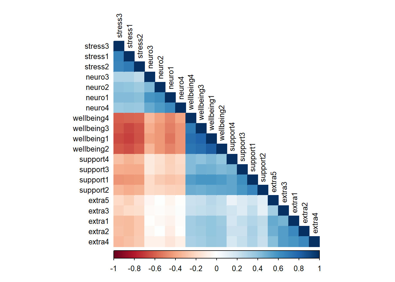
##            vars   n mean   sd median trimmed  mad min max range  skew kurtosis
## extra1        1 500 3.09 0.99      3    3.07 1.48   1   7     6  0.15     0.02
## extra2        2 500 3.09 1.02      3    3.09 1.48   1   6     5 -0.06    -0.43
## extra3        3 500 3.10 1.04      3    3.06 1.48   1   6     5  0.13    -0.39
## extra4        4 500 3.09 1.07      3    3.06 1.48   1   6     5  0.16    -0.34
## extra5        5 500 3.13 0.99      3    3.12 1.48   1   6     5 -0.03    -0.26
## neuro1        6 500 3.05 1.05      3    3.04 1.48   1   6     5  0.11    -0.19
## neuro2        7 500 3.06 1.06      3    3.06 1.48   1   6     5 -0.03    -0.46
## neuro3        8 500 2.98 0.97      3    2.98 1.48   1   6     5  0.06    -0.33
## neuro4        9 500 3.04 1.02      3    3.04 1.48   1   6     5  0.02    -0.27
## support1     10 500 3.09 1.06      3    3.08 1.48   1   6     5  0.06    -0.33
## support2     11 500 3.08 1.05      3    3.09 1.48   1   6     5 -0.06    -0.31
## support3     12 500 3.06 0.91      3    3.10 1.48   1   5     4 -0.29    -0.24
## support4     13 500 3.04 1.00      3    3.04 1.48   1   6     5 -0.02    -0.38
## stress1      14 500 2.97 1.13      3    2.97 1.48   1   7     6  0.15    -0.19
## stress2      15 500 3.01 1.10      3    3.01 1.48   1   6     5  0.09    -0.24
## stress3      16 500 3.00 1.11      3    3.01 1.48   1   6     5 -0.02    -0.48
## wellbeing1   17 500 3.08 1.41      3    3.03 1.48   1   7     6  0.32    -0.43
## wellbeing2   18 500 3.13 1.33      3    3.12 1.48   1   7     6  0.18    -0.56
## wellbeing3   19 500 3.08 1.32      3    3.06 1.48   1   7     6  0.21    -0.45
## wellbeing4   20 500 3.09 1.34      3    3.06 1.48   1   7     6  0.29    -0.52
##              se
## extra1     0.04
## extra2     0.05
## extra3     0.05
## extra4     0.05
## extra5     0.04
## neuro1     0.05
## neuro2     0.05
## neuro3     0.04
## neuro4     0.05
## support1   0.05
## support2   0.05
## support3   0.04
## support4   0.04
## stress1    0.05
## stress2    0.05
## stress3    0.05
## wellbeing1 0.06
## wellbeing2 0.06
## wellbeing3 0.06
## wellbeing4 0.06## NULL# Reliability analysis for each construct
alpha_extra <- alpha(sem_data[, paste0("extra", 1:5)])
alpha_neuro <- alpha(sem_data[, paste0("neuro", 1:4)])
alpha_support <- alpha(sem_data[, paste0("support", 1:4)])
alpha_stress <- alpha(sem_data[, paste0("stress", 1:3)])
alpha_wellbeing <- alpha(sem_data[, paste0("wellbeing", 1:4)])
print(paste("Extraversion Cronbach's α:", round(alpha_extra$total$std.alpha, 3)))## [1] "Extraversion Cronbach's α: 0.845"## [1] "Neuroticism Cronbach's α: 0.835"## [1] "Social Support Cronbach's α: 0.838"## [1] "Stress Cronbach's α: 0.863"## [1] "Well-being Cronbach's α: 0.927"2.15 Step 1: Confirmatory Factor Analysis (CFA)
First, we’ll test the measurement model to ensure our latent variables are well-defined.
# Define the measurement model
measurement_model <- '
  # Latent variable definitions
  extraversion =~ extra1 + extra2 + extra3 + extra4 + extra5
  neuroticism =~ neuro1 + neuro2 + neuro3 + neuro4
  social_support =~ support1 + support2 + support3 + support4
  stress =~ stress1 + stress2 + stress3
  wellbeing =~ wellbeing1 + wellbeing2 + wellbeing3 + wellbeing4
'

# Fit the CFA model
cfa_fit <- cfa(measurement_model, data = sem_data, estimator = "MLR")

# Model summary
summary(cfa_fit, fit.measures = TRUE, standardized = TRUE)
## lavaan 0.6-19 ended normally after 44 iterations
##
## Estimator ML
## Optimization method NLMINB
## Number of model parameters 50
##
## Number of observations 500
##
## Model Test User Model:
## Standard Scaled
## Test Statistic 172.554 172.351
## Degrees of freedom 160 160
## P-value (Chi-square) 0.235 0.239
## Scaling correction factor 1.001
## Yuan-Bentler correction (Mplus variant)
##
## Model Test Baseline Model:
##
## Test statistic 6166.734 6108.463
## Degrees of freedom 190 190
## P-value 0.000 0.000
## Scaling correction factor 1.010
##
## User Model versus Baseline Model:
##
## Comparative Fit Index (CFI) 0.998 0.998
## Tucker-Lewis Index (TLI) 0.998 0.998
##
## Robust Comparative Fit Index (CFI) 0.998
## Robust Tucker-Lewis Index (TLI) 0.998
##
## Loglikelihood and Information Criteria:
##
## Loglikelihood user model (H0) -12043.684 -12043.684
## Scaling correction factor 0.967
## for the MLR correction
## Loglikelihood unrestricted model (H1) -11957.407 -11957.407
## Scaling correction factor 0.993
## for the MLR correction
##
## Akaike (AIC) 24187.368 24187.368
## Bayesian (BIC) 24398.098 24398.098
## Sample-size adjusted Bayesian (SABIC) 24239.395 24239.395
##
## Root Mean Square Error of Approximation:
##
## RMSEA 0.013 0.012
## 90 Percent confidence interval - lower 0.000 0.000
## 90 Percent confidence interval - upper 0.025 0.025
## P-value H_0: RMSEA <= 0.050 1.000 1.000
## P-value H_0: RMSEA >= 0.080 0.000 0.000
##
## Robust RMSEA 0.012
## 90 Percent confidence interval - lower 0.000
## 90 Percent confidence interval - upper 0.025
## P-value H_0: Robust RMSEA <= 0.050 1.000
## P-value H_0: Robust RMSEA >= 0.080 0.000
##
## Standardized Root Mean Square Residual:
##
## SRMR 0.026 0.026
##
## Parameter Estimates:
##
## Standard errors Sandwich
## Information bread Observed
## Observed information based on Hessian
##
## Latent Variables:
## Estimate Std.Err z-value P(>|z|) Std.lv Std.all
## extraversion =~
## extra1 1.000 0.763 0.774
## extra2 1.119 0.060 18.674 0.000 0.853 0.841
## extra3 0.882 0.064 13.805 0.000 0.673 0.647
## extra4 1.082 0.066 16.314 0.000 0.825 0.771
## extra5 0.753 0.056 13.370 0.000 0.574 0.583
## neuroticism =~
## neuro1 1.000 0.889 0.849
## neuro2 0.869 0.050 17.322 0.000 0.772 0.726
## neuro3 0.713 0.046 15.356 0.000 0.634 0.656
## neuro4 0.876 0.048 18.114 0.000 0.779 0.761
## social_support =~
## support1 1.000 0.893 0.846
## support2 0.924 0.050 18.657 0.000 0.826 0.789
## support3 0.743 0.041 18.254 0.000 0.664 0.730
## support4 0.717 0.050 14.470 0.000 0.640 0.639
## stress =~
## stress1 1.000 0.966 0.853
## stress2 0.921 0.041 22.250 0.000 0.890 0.812
## stress3 0.923 0.045 20.546 0.000 0.892 0.806
## wellbeing =~
## wellbeing1 1.000 1.298 0.922
## wellbeing2 0.899 0.025 36.657 0.000 1.167 0.880
## wellbeing3 0.882 0.028 31.319 0.000 1.144 0.869
## wellbeing4 0.846 0.031 27.616 0.000 1.098 0.818
##
## Covariances:
## Estimate Std.Err z-value P(>|z|) Std.lv Std.all
## extraversion ~~
## neuroticism -0.059 0.036 -1.657 0.098 -0.087 -0.087
## social_support 0.275 0.040 6.857 0.000 0.404 0.404
## stress -0.319 0.043 -7.398 0.000 -0.433 -0.433
## wellbeing 0.504 0.053 9.565 0.000 0.510 0.510
## neuroticism ~~
## social_support -0.295 0.042 -7.039 0.000 -0.372 -0.372
## stress 0.519 0.051 10.242 0.000 0.604 0.604
## wellbeing -0.768 0.066 -11.681 0.000 -0.666 -0.666
## social_support ~~
## stress -0.515 0.052 -9.962 0.000 -0.597 -0.597
## wellbeing 0.860 0.068 12.678 0.000 0.742 0.742
## stress ~~
## wellbeing -1.091 0.076 -14.347 0.000 -0.870 -0.870
##
## Variances:
## Estimate Std.Err z-value P(>|z|) Std.lv Std.all
## .extra1 0.389 0.035 11.225 0.000 0.389 0.401
## .extra2 0.302 0.030 9.985 0.000 0.302 0.293
## .extra3 0.628 0.048 13.190 0.000 0.628 0.581
## .extra4 0.463 0.037 12.576 0.000 0.463 0.405
## .extra5 0.640 0.043 14.846 0.000 0.640 0.660
## .neuro1 0.306 0.031 9.841 0.000 0.306 0.279
## .neuro2 0.534 0.042 12.775 0.000 0.534 0.473
## .neuro3 0.530 0.040 13.260 0.000 0.530 0.569
## .neuro4 0.441 0.033 13.262 0.000 0.441 0.421
## .support1 0.317 0.031 10.258 0.000 0.317 0.284
## .support2 0.414 0.038 10.984 0.000 0.414 0.378
## .support3 0.386 0.030 12.992 0.000 0.386 0.467
## .support4 0.595 0.038 15.452 0.000 0.595 0.592
## .stress1 0.350 0.032 11.070 0.000 0.350 0.273
## .stress2 0.410 0.035 11.690 0.000 0.410 0.341
## .stress3 0.429 0.036 12.027 0.000 0.429 0.351
## .wellbeing1 0.296 0.032 9.159 0.000 0.296 0.149
## .wellbeing2 0.398 0.032 12.626 0.000 0.398 0.226
## .wellbeing3 0.423 0.029 14.539 0.000 0.423 0.244
## .wellbeing4 0.595 0.043 13.969 0.000 0.595 0.330
## extraversion 0.582 0.057 10.180 0.000 1.000 1.000
## neuroticism 0.790 0.069 11.496 0.000 1.000 1.000
## social_support 0.798 0.066 12.104 0.000 1.000 1.000
## stress 0.933 0.077 12.048 0.000 1.000 1.000
## wellbeing 1.684 0.112 14.988 0.000 1.000 1.000# Model fit indices
fit_indices <- fitMeasures(cfa_fit, c("chisq", "df", "pvalue", "cfi", "tli",
"rmsea", "rmsea.ci.lower", "rmsea.ci.upper",
"srmr", "aic", "bic"))
print(fit_indices)## chisq df pvalue cfi tli
## 172.554 160.000 0.235 0.998 0.998
## rmsea rmsea.ci.lower rmsea.ci.upper srmr aic
## 0.013 0.000 0.025 0.026 24187.368
## bic
## 24398.0982.16 Step 2: Full Structural Equation Model
Now we’ll test the full structural model with hypothesized relationships.
# Define the full SEM model
structural_model <- '
  # Measurement model
  extraversion =~ extra1 + extra2 + extra3 + extra4 + extra5
  neuroticism =~ neuro1 + neuro2 + neuro3 + neuro4
  social_support =~ support1 + support2 + support3 + support4
  stress =~ stress1 + stress2 + stress3
  wellbeing =~ wellbeing1 + wellbeing2 + wellbeing3 + wellbeing4

  # Structural model
  social_support ~ extraversion + neuroticism
  stress ~ extraversion + neuroticism + social_support
  wellbeing ~ extraversion + neuroticism + social_support + stress
'

# Fit the SEM model
sem_fit <- sem(structural_model, data = sem_data, estimator = "MLR")

# Model summary
summary(sem_fit, fit.measures = TRUE, standardized = TRUE, rsquare = TRUE)
## lavaan 0.6-19 ended normally after 33 iterations
##
## Estimator ML
## Optimization method NLMINB
## Number of model parameters 50
##
## Number of observations 500
##
## Model Test User Model:
## Standard Scaled
## Test Statistic 172.554 172.351
## Degrees of freedom 160 160
## P-value (Chi-square) 0.235 0.239
## Scaling correction factor 1.001
## Yuan-Bentler correction (Mplus variant)
##
## Model Test Baseline Model:
##
## Test statistic 6166.734 6108.463
## Degrees of freedom 190 190
## P-value 0.000 0.000
## Scaling correction factor 1.010
##
## User Model versus Baseline Model:
##
## Comparative Fit Index (CFI) 0.998 0.998
## Tucker-Lewis Index (TLI) 0.998 0.998
##
## Robust Comparative Fit Index (CFI) 0.998
## Robust Tucker-Lewis Index (TLI) 0.998
##
## Loglikelihood and Information Criteria:
##
## Loglikelihood user model (H0) -12043.684 -12043.684
## Scaling correction factor 0.967
## for the MLR correction
## Loglikelihood unrestricted model (H1) -11957.407 -11957.407
## Scaling correction factor 0.993
## for the MLR correction
##
## Akaike (AIC) 24187.368 24187.368
## Bayesian (BIC) 24398.098 24398.098
## Sample-size adjusted Bayesian (SABIC) 24239.395 24239.395
##
## Root Mean Square Error of Approximation:
##
## RMSEA 0.013 0.012
## 90 Percent confidence interval - lower 0.000 0.000
## 90 Percent confidence interval - upper 0.025 0.025
## P-value H_0: RMSEA <= 0.050 1.000 1.000
## P-value H_0: RMSEA >= 0.080 0.000 0.000
##
## Robust RMSEA 0.012
## 90 Percent confidence interval - lower 0.000
## 90 Percent confidence interval - upper 0.025
## P-value H_0: Robust RMSEA <= 0.050 1.000
## P-value H_0: Robust RMSEA >= 0.080 0.000
##
## Standardized Root Mean Square Residual:
##
## SRMR 0.026 0.026
##
## Parameter Estimates:
##
## Standard errors Sandwich
## Information bread Observed
## Observed information based on Hessian
##
## Latent Variables:
## Estimate Std.Err z-value P(>|z|) Std.lv Std.all
## extraversion =~
## extra1 1.000 0.763 0.774
## extra2 1.119 0.060 18.674 0.000 0.853 0.841
## extra3 0.882 0.064 13.805 0.000 0.673 0.647
## extra4 1.082 0.066 16.314 0.000 0.825 0.771
## extra5 0.753 0.056 13.370 0.000 0.574 0.583
## neuroticism =~
## neuro1 1.000 0.889 0.849
## neuro2 0.869 0.050 17.322 0.000 0.772 0.726
## neuro3 0.713 0.046 15.356 0.000 0.634 0.656
## neuro4 0.876 0.048 18.114 0.000 0.779 0.761
## social_support =~
## support1 1.000 0.893 0.846
## support2 0.924 0.050 18.657 0.000 0.826 0.789
## support3 0.743 0.041 18.254 0.000 0.664 0.730
## support4 0.717 0.050 14.470 0.000 0.640 0.639
## stress =~
## stress1 1.000 0.966 0.853
## stress2 0.921 0.041 22.250 0.000 0.890 0.812
## stress3 0.923 0.045 20.546 0.000 0.892 0.806
## wellbeing =~
## wellbeing1 1.000 1.298 0.922
## wellbeing2 0.899 0.025 36.657 0.000 1.167 0.880
## wellbeing3 0.882 0.028 31.319 0.000 1.144 0.869
## wellbeing4 0.846 0.031 27.616 0.000 1.098 0.818
##
## Regressions:
## Estimate Std.Err z-value P(>|z|) Std.lv Std.all
## social_support ~
## extraversion 0.439 0.057 7.728 0.000 0.375 0.375
## neuroticism -0.340 0.048 -7.167 0.000 -0.339 -0.339
## stress ~
## extraversion -0.334 0.058 -5.789 0.000 -0.263 -0.263
## neuroticism 0.503 0.051 9.883 0.000 0.463 0.463
## social_support -0.344 0.054 -6.382 0.000 -0.318 -0.318
## wellbeing ~
## extraversion 0.281 0.053 5.344 0.000 0.165 0.165
## neuroticism -0.381 0.057 -6.746 0.000 -0.261 -0.261
## social_support 0.442 0.045 9.724 0.000 0.304 0.304
## stress -0.617 0.069 -8.986 0.000 -0.460 -0.460
##
## Covariances:
## Estimate Std.Err z-value P(>|z|) Std.lv Std.all
## extraversion ~~
## neuroticism -0.059 0.036 -1.657 0.098 -0.087 -0.087
##
## Variances:
## Estimate Std.Err z-value P(>|z|) Std.lv Std.all
## .extra1 0.389 0.035 11.225 0.000 0.389 0.401
## .extra2 0.302 0.030 9.985 0.000 0.302 0.293
## .extra3 0.628 0.048 13.190 0.000 0.628 0.581
## .extra4 0.463 0.037 12.576 0.000 0.463 0.405
## .extra5 0.640 0.043 14.846 0.000 0.640 0.660
## .neuro1 0.306 0.031 9.841 0.000 0.306 0.279
## .neuro2 0.534 0.042 12.775 0.000 0.534 0.473
## .neuro3 0.530 0.040 13.260 0.000 0.530 0.569
## .neuro4 0.441 0.033 13.262 0.000 0.441 0.421
## .support1 0.317 0.031 10.258 0.000 0.317 0.284
## .support2 0.414 0.038 10.984 0.000 0.414 0.378
## .support3 0.386 0.030 12.992 0.000 0.386 0.467
## .support4 0.595 0.038 15.452 0.000 0.595 0.592
## .stress1 0.350 0.032 11.070 0.000 0.350 0.273
## .stress2 0.410 0.035 11.690 0.000 0.410 0.341
## .stress3 0.429 0.036 12.027 0.000 0.429 0.351
## .wellbeing1 0.296 0.032 9.159 0.000 0.296 0.149
## .wellbeing2 0.398 0.032 12.626 0.000 0.398 0.226
## .wellbeing3 0.423 0.029 14.539 0.000 0.423 0.244
## .wellbeing4 0.595 0.043 13.969 0.000 0.595 0.330
## extraversion 0.582 0.057 10.180 0.000 1.000 1.000
## neuroticism 0.790 0.069 11.496 0.000 1.000 1.000
## .social_support 0.576 0.050 11.534 0.000 0.723 0.723
## .stress 0.389 0.041 9.378 0.000 0.417 0.417
## .wellbeing 0.196 0.027 7.200 0.000 0.116 0.116
##
## R-Square:
## Estimate
## extra1 0.599
## extra2 0.707
## extra3 0.419
## extra4 0.595
## extra5 0.340
## neuro1 0.721
## neuro2 0.527
## neuro3 0.431
## neuro4 0.579
## support1 0.716
## support2 0.622
## support3 0.533
## support4 0.408
## stress1 0.727
## stress2 0.659
## stress3 0.649
## wellbeing1 0.851
## wellbeing2 0.774
## wellbeing3 0.756
## wellbeing4 0.670
## social_support 0.277
## stress 0.583
## wellbeing 0.884## [1] "Support for lavaan not fully implemented yet :("2.17 Model Diagnostics and Fit Assessment
# Comprehensive fit measures
fit_measures_sem <- fitMeasures(sem_fit, c("chisq", "df", "pvalue", "cfi", "tli",
                                           "rmsea", "rmsea.ci.lower", "rmsea.ci.upper",
                                           "srmr", "aic", "bic"))

# Create a fit measures table
fit_table <- data.frame(
  Measure = names(fit_measures_sem),
  Value = round(fit_measures_sem, 3),
  Interpretation = c(
    "Model Chi-square", "Degrees of freedom", "P-value",
    "Comparative Fit Index (>0.95 excellent)",
    "Tucker-Lewis Index (>0.95 excellent)",
    "RMSEA (<0.06 excellent)", "RMSEA CI Lower", "RMSEA CI Upper",
    "SRMR (<0.08 good)", "AIC (lower is better)", "BIC (lower is better)"
  )
)

print(fit_table)
## Measure Value Interpretation
## chisq chisq 172.554 Model Chi-square
## df df 160.000 Degrees of freedom
## pvalue pvalue 0.235 P-value
## cfi cfi 0.998 Comparative Fit Index (>0.95 excellent)
## tli tli 0.998 Tucker-Lewis Index (>0.95 excellent)
## rmsea rmsea 0.013 RMSEA (<0.06 excellent)
## rmsea.ci.lower rmsea.ci.lower 0.000 RMSEA CI Lower
## rmsea.ci.upper rmsea.ci.upper 0.025 RMSEA CI Upper
## srmr srmr 0.026 SRMR (<0.08 good)
## aic aic 24187.368 AIC (lower is better)
## bic bic 24398.098 BIC (lower is better)# Modification indices
mod_indices <- modificationIndices(sem_fit, sort = TRUE, maximum.number = 10)
print("Top 10 Modification Indices:")## [1] "Top 10 Modification Indices:"## lhs op rhs mi epc sepc.lv sepc.all sepc.nox
## 173 extra3 ~~ extra4 9.912 0.096 0.096 0.178 0.178
## 139 extra1 ~~ extra5 7.295 0.074 0.074 0.148 0.148
## 180 extra3 ~~ support2 7.163 -0.072 -0.072 -0.141 -0.141
## 60 extraversion =~ support1 6.262 0.134 0.102 0.097 0.097
## 113 stress =~ support2 5.597 0.124 0.120 0.115 0.115
## 182 extra3 ~~ support4 5.111 0.068 0.068 0.111 0.111
## 74 neuroticism =~ extra4 4.923 -0.093 -0.083 -0.077 -0.077
## 137 extra1 ~~ extra3 4.633 -0.060 -0.060 -0.122 -0.122
## 129 wellbeing =~ support1 4.555 0.106 0.138 0.130 0.130
## 56 extraversion =~ neuro1 4.471 -0.099 -0.076 -0.072 -0.072# Residuals
residuals_sem <- residuals(sem_fit, type = "cor")
print("Correlation residuals (should be small):")## [1] "Correlation residuals (should be small):"if(is.matrix(residuals_sem$cor) && is.numeric(residuals_sem$cor)) {
print(round(residuals_sem$cor[1:5, 1:5], 3))
} else {
print("Residual correlation matrix:")
print(residuals_sem$cor[1:5, 1:5])
}## [1] "Residual correlation matrix:"
## NULL2.18 Visualization of the SEM Model
# Plot the SEM model with standardized coefficients
semPaths(sem_fit, what = "std", whatLabels = "std", style = "lisrel",
         layout = "tree2", rotation = 2, curve = 1,
         sizeLat = 8, sizeMan = 4, edge.label.cex = 0.8)
title("Structural Equation Model: Personality, Support, Stress, and Well-being")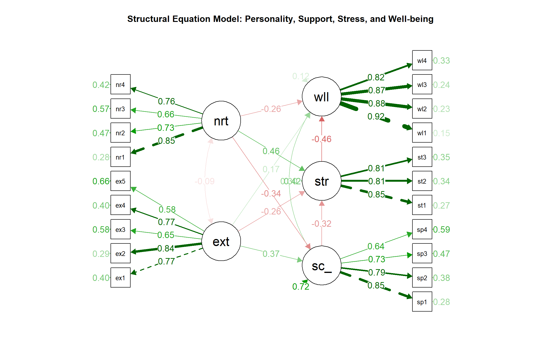
# Alternative visualization with path coefficients
semPaths(sem_fit, what = "par", whatLabels = "par", style = "lisrel",
         layout = "tree2", rotation = 2, curve = 1,
         sizeLat = 8, sizeMan = 4, edge.label.cex = 0.8)
title("SEM Model with Parameter Estimates")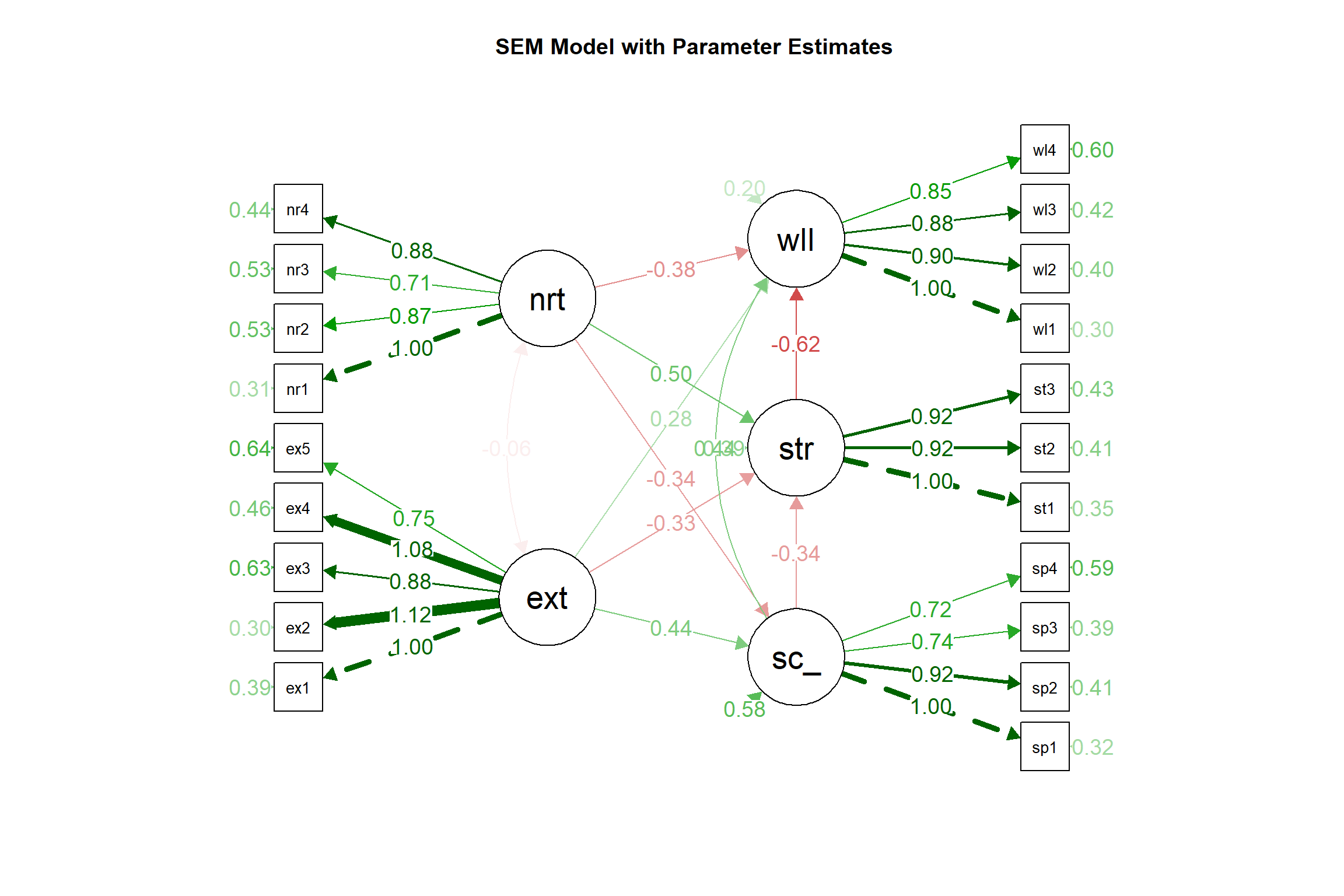
2.19 Effect Decomposition and Mediation Analysis
# Calculate direct, indirect, and total effects
effects <- parameterEstimates(sem_fit, standardized = TRUE)

# Extract structural parameters
structural_params <- effects[effects$op == "~", ]
print("Structural Parameters (Direct Effects):")
## [1] "Structural Parameters (Direct Effects):"## lhs rhs est se pvalue std.all
## 21 social_support extraversion 0.439 0.057 0 0.375
## 22 social_support neuroticism -0.340 0.048 0 -0.339
## 23 stress extraversion -0.334 0.058 0 -0.263
## 24 stress neuroticism 0.503 0.051 0 0.463
## 25 stress social_support -0.344 0.054 0 -0.318
## 26 wellbeing extraversion 0.281 0.053 0 0.165
## 27 wellbeing neuroticism -0.381 0.057 0 -0.261
## 28 wellbeing social_support 0.442 0.045 0 0.304
## 29 wellbeing stress -0.617 0.069 0 -0.460# Calculate indirect effects using lavaan
indirect_model <- '
# Measurement model
extraversion =~ extra1 + extra2 + extra3 + extra4 + extra5
neuroticism =~ neuro1 + neuro2 + neuro3 + neuro4
social_support =~ support1 + support2 + support3 + support4
stress =~ stress1 + stress2 + stress3
wellbeing =~ wellbeing1 + wellbeing2 + wellbeing3 + wellbeing4
# Structural model
social_support ~ a1*extraversion + a2*neuroticism
stress ~ b1*extraversion + b2*neuroticism + b3*social_support
wellbeing ~ c1*extraversion + c2*neuroticism + c3*social_support + c4*stress
# Indirect effects
ext_well_via_support := a1 * c3
ext_well_via_stress := b1 * c4
ext_well_via_support_stress := a1 * b3 * c4
neuro_well_via_support := a2 * c3
neuro_well_via_stress := b2 * c4
neuro_well_via_support_stress := a2 * b3 * c4
support_well_via_stress := b3 * c4
# Total indirect effects
ext_well_total_indirect := ext_well_via_support + ext_well_via_stress + ext_well_via_support_stress
neuro_well_total_indirect := neuro_well_via_support + neuro_well_via_stress + neuro_well_via_support_stress
'
# Fit model with indirect effects
indirect_fit <- sem(indirect_model, data = sem_data, estimator = "MLR")
# Extract indirect effects
indirect_effects <- parameterEstimates(indirect_fit, standardized = TRUE)
indirect_results <- indirect_effects[grep(":=", indirect_effects$op), ]
print("Indirect Effects:")## [1] "Indirect Effects:"## lhs est se pvalue std.all
## 56 ext_well_via_support 0.194 0.032 0 0.114
## 57 ext_well_via_stress 0.206 0.043 0 0.121
## 58 ext_well_via_support_stress 0.093 0.020 0 0.055
## 59 neuro_well_via_support -0.150 0.025 0 -0.103
## 60 neuro_well_via_stress -0.310 0.044 0 -0.213
## 61 neuro_well_via_support_stress -0.072 0.016 0 -0.050
## 62 support_well_via_stress 0.212 0.039 0 0.146
## 63 ext_well_total_indirect 0.493 0.056 0 0.290
## 64 neuro_well_total_indirect -0.533 0.055 0 -0.3652.20 Bootstrap Confidence Intervals for Indirect Effects
# Bootstrap confidence intervals for more robust inference
# Note: Bootstrap requires ML estimator, not MLR
bootstrap_fit <- sem(indirect_model, data = sem_data, estimator = "ML",
                     se = "bootstrap", bootstrap = 500)

# Bootstrap results for indirect effects
bootstrap_results <- parameterEstimates(bootstrap_fit, standardized = TRUE,
                                        boot.ci.type = "perc")
bootstrap_indirect <- bootstrap_results[grep(":=", bootstrap_results$op), ]
print("Bootstrap Confidence Intervals for Indirect Effects:")
## [1] "Bootstrap Confidence Intervals for Indirect Effects:"## lhs est se ci.lower ci.upper pvalue
## 56 ext_well_via_support 0.194 0.031 0.132 0.259 0
## 57 ext_well_via_stress 0.206 0.044 0.129 0.297 0
## 58 ext_well_via_support_stress 0.093 0.020 0.057 0.135 0
## 59 neuro_well_via_support -0.150 0.025 -0.201 -0.103 0
## 60 neuro_well_via_stress -0.310 0.043 -0.402 -0.235 0
## 61 neuro_well_via_support_stress -0.072 0.017 -0.113 -0.044 0
## 62 support_well_via_stress 0.212 0.040 0.133 0.295 0
## 63 ext_well_total_indirect 0.493 0.056 0.392 0.622 0
## 64 neuro_well_total_indirect -0.533 0.056 -0.648 -0.430 02.21 Model Comparison: Alternative Models
# Test alternative model without direct paths from personality to well-being
alternative_model <- '
  # Measurement model
  extraversion =~ extra1 + extra2 + extra3 + extra4 + extra5
  neuroticism =~ neuro1 + neuro2 + neuro3 + neuro4
  social_support =~ support1 + support2 + support3 + support4
  stress =~ stress1 + stress2 + stress3
  wellbeing =~ wellbeing1 + wellbeing2 + wellbeing3 + wellbeing4

  # Structural model (mediation only)
  social_support ~ extraversion + neuroticism
  stress ~ extraversion + neuroticism + social_support
  wellbeing ~ social_support + stress
'

# Fit alternative model
alt_fit <- sem(alternative_model, data = sem_data, estimator = "MLR")

# Compare models
anova(alt_fit, sem_fit)
##
## Scaled Chi-Squared Difference Test (method = "satorra.bentler.2001")
##
## lavaan->lavTestLRT():
## lavaan NOTE: The "Chisq" column contains standard test statistics, not the
## robust test that should be reported per model. A robust difference test is
## a function of two standard (not robust) statistics.
## Df AIC BIC Chisq Chisq diff Df diff Pr(>Chisq)
## sem_fit 160 24187 24398 172.55
## alt_fit 162 24240 24442 228.80 65.354 2 6.436e-15 ***
## ---
## Signif. codes: 0 '***' 0.001 '**' 0.01 '*' 0.05 '.' 0.1 ' ' 1# Compare fit indices
comparison <- data.frame(
Model = c("Full Model", "Mediation Only"),
AIC = c(AIC(sem_fit), AIC(alt_fit)),
BIC = c(BIC(sem_fit), BIC(alt_fit)),
CFI = c(fitMeasures(sem_fit, "cfi"), fitMeasures(alt_fit, "cfi")),
RMSEA = c(fitMeasures(sem_fit, "rmsea"), fitMeasures(alt_fit, "rmsea"))
)
print(comparison)## Model AIC BIC CFI RMSEA
## 1 Full Model 24187.37 24398.10 0.9978995 0.01252712
## 2 Mediation Only 24239.61 24441.91 0.9888241 0.028716492.22 Power Analysis for SEM
# Power analysis using semTools
# Note: SSpower requires a population model specification

# Alternative approach: Use simulation-based power analysis
# First, extract the population parameters from our fitted model
pop_params <- parameterEstimates(sem_fit, standardized = FALSE)

# Define population model using the fitted parameters
pop_model <- '
  # Measurement model
  extraversion =~ 0.8*extra1 + 0.9*extra2 + 0.7*extra3 + 0.8*extra4 + 0.6*extra5
  neuroticism =~ 0.9*neuro1 + 0.8*neuro2 + 0.7*neuro3 + 0.8*neuro4
  social_support =~ 0.9*support1 + 0.8*support2 + 0.8*support3 + 0.7*support4
  stress =~ 0.9*stress1 + 0.8*stress2 + 0.8*stress3
  wellbeing =~ 0.9*wellbeing1 + 0.8*wellbeing2 + 0.8*wellbeing3 + 0.7*wellbeing4

  # Structural model (using approximate population values)
  social_support ~ 0.35*extraversion + -0.25*neuroticism
  stress ~ -0.25*extraversion + 0.45*neuroticism + -0.35*social_support
  wellbeing ~ 0.25*extraversion + -0.35*neuroticism + 0.45*social_support + -0.55*stress
'

# Simple power analysis using effect sizes
# Calculate power for key structural paths using approximate formulas
print("Power Analysis for Key Structural Paths:")
## [1] "Power Analysis for Key Structural Paths:"## [1] "========================================"# Function to calculate approximate power for regression coefficients
calc_power <- function(effect_size, n, alpha = 0.05) {
# Convert effect size to t-statistic
t_stat <- effect_size * sqrt(n - 2) / sqrt(1 - effect_size^2)
# Calculate power using t-distribution
t_crit <- qt(1 - alpha/2, n - 2)
power <- 1 - pt(t_crit, n - 2, ncp = abs(t_stat)) + pt(-t_crit, n - 2, ncp = abs(t_stat))
return(power)
}
# Calculate power for standardized effects
n_current <- nrow(sem_data)
# Get standardized coefficients (effect sizes)
std_estimates <- standardizedSolution(sem_fit)
structural_std <- std_estimates[std_estimates$op == "~", ]
key_effects <- structural_std[c(1:7), c("lhs", "rhs", "est.std")]
for(i in seq_len(nrow(key_effects))) {
effect <- key_effects[i, "est.std"]
if(!is.na(effect) && abs(effect) > 0.001) {
power <- calc_power(effect, n_current)
cat(sprintf("%s -> %s: Effect = %.3f, Power = %.3f\n",
key_effects[i, "rhs"], key_effects[i, "lhs"], effect, power))
}
}## extraversion -> social_support: Effect = 0.375, Power = 1.000
## neuroticism -> social_support: Effect = -0.339, Power = 1.000
## extraversion -> stress: Effect = -0.263, Power = 1.000
## neuroticism -> stress: Effect = 0.463, Power = 1.000
## social_support -> stress: Effect = -0.318, Power = 1.000
## extraversion -> wellbeing: Effect = 0.165, Power = 0.962
## neuroticism -> wellbeing: Effect = -0.261, Power = 1.000## [1] "\nSample Size Requirements for 80% Power:"## [1] "======================================"target_power <- 0.80
alpha <- 0.05
for(i in seq_len(nrow(key_effects))) {
effect <- key_effects[i, "est.std"]
if(!is.na(effect) && abs(effect) > 0.001) {
# Approximate sample size for desired power
# Using Cohen's formula for correlation/regression
z_alpha <- qnorm(1 - alpha/2)
z_beta <- qnorm(target_power)
n_needed <- ((z_alpha + z_beta)^2 / effect^2) + 3
cat(sprintf("%s -> %s: Effect = %.3f, N needed = %.0f\n",
key_effects[i, "rhs"], key_effects[i, "lhs"], effect, n_needed))
}
}## extraversion -> social_support: Effect = 0.375, N needed = 59
## neuroticism -> social_support: Effect = -0.339, N needed = 71
## extraversion -> stress: Effect = -0.263, N needed = 116
## neuroticism -> stress: Effect = 0.463, N needed = 40
## social_support -> stress: Effect = -0.318, N needed = 81
## extraversion -> wellbeing: Effect = 0.165, N needed = 291
## neuroticism -> wellbeing: Effect = -0.261, N needed = 118## [1] "\nModel Fit and Power Assessment:"## [1] "==============================="## Current sample size: 500## Model degrees of freedom: 160## Chi-square p-value: 0.235cat(sprintf("RMSEA: %.3f (90%% CI: %.3f - %.3f)\n",
fitMeasures(sem_fit, "rmsea"),
fitMeasures(sem_fit, "rmsea.ci.lower"),
fitMeasures(sem_fit, "rmsea.ci.upper")))## RMSEA: 0.013 (90% CI: 0.000 - 0.025)# Rule of thumb: 10-20 observations per parameter
n_params <- length(coef(sem_fit))
cat(sprintf("Number of free parameters: %d\n", n_params))## Number of free parameters: 50## Observations per parameter: 10.0## Recommended minimum sample size (10:1 rule): 500## Recommended optimal sample size (20:1 rule): 10002.23 Effect Sizes and Practical Significance
# R-squared for endogenous variables
r_squared <- inspect(sem_fit, "r2")
print("R-squared values for endogenous variables:")
## [1] "R-squared values for endogenous variables:"## extra1 extra2 extra3 extra4 extra5
## 0.599 0.707 0.419 0.595 0.340
## neuro1 neuro2 neuro3 neuro4 support1
## 0.721 0.527 0.431 0.579 0.716
## support2 support3 support4 stress1 stress2
## 0.622 0.533 0.408 0.727 0.659
## stress3 wellbeing1 wellbeing2 wellbeing3 wellbeing4
## 0.649 0.851 0.774 0.756 0.670
## social_support stress wellbeing
## 0.277 0.583 0.884# Standardized coefficients (effect sizes) - already calculated in power analysis
print("Standardized coefficients (effect sizes):")## [1] "Standardized coefficients (effect sizes):"## lhs rhs est.std pvalue
## 21 social_support extraversion 0.375 0
## 22 social_support neuroticism -0.339 0
## 23 stress extraversion -0.263 0
## 24 stress neuroticism 0.463 0
## 25 stress social_support -0.318 0
## 26 wellbeing extraversion 0.165 0
## 27 wellbeing neuroticism -0.261 0
## 28 wellbeing social_support 0.304 0
## 29 wellbeing stress -0.460 0# Cohen's guidelines for effect sizes:
# Small: 0.10, Medium: 0.30, Large: 0.50
effect_size_interpretation <- function(coef) {
abs_coef <- abs(coef)
if (abs_coef < 0.10) return("Negligible")
else if (abs_coef < 0.30) return("Small")
else if (abs_coef < 0.50) return("Medium")
else return("Large")
}
structural_std$effect_size <- sapply(structural_std$est.std, effect_size_interpretation)
print("Effect size interpretations:")## [1] "Effect size interpretations:"## lhs rhs est.std effect_size
## 21 social_support extraversion 0.375 Medium
## 22 social_support neuroticism -0.339 Medium
## 23 stress extraversion -0.263 Small
## 24 stress neuroticism 0.463 Medium
## 25 stress social_support -0.318 Medium
## 26 wellbeing extraversion 0.165 Small
## 27 wellbeing neuroticism -0.261 Small
## 28 wellbeing social_support 0.304 Medium
## 29 wellbeing stress -0.460 Medium2.24 Interpretation of Results
2.24.1 Measurement Model Quality
# Factor loadings
loadings <- parameterEstimates(sem_fit, standardized = TRUE)
factor_loadings <- loadings[loadings$op == "=~", ]
print("Standardized Factor Loadings:")
## [1] "Standardized Factor Loadings:"## lhs rhs std.all
## 1 extraversion extra1 0.774
## 2 extraversion extra2 0.841
## 3 extraversion extra3 0.647
## 4 extraversion extra4 0.771
## 5 extraversion extra5 0.583
## 6 neuroticism neuro1 0.849
## 7 neuroticism neuro2 0.726
## 8 neuroticism neuro3 0.656
## 9 neuroticism neuro4 0.761
## 10 social_support support1 0.846
## 11 social_support support2 0.789
## 12 social_support support3 0.730
## 13 social_support support4 0.639
## 14 stress stress1 0.853
## 15 stress stress2 0.812
## 16 stress stress3 0.806
## 17 wellbeing wellbeing1 0.922
## 18 wellbeing wellbeing2 0.880
## 19 wellbeing wellbeing3 0.869
## 20 wellbeing wellbeing4 0.818# Composite reliability
reliability <- semTools::reliability(sem_fit)
print("Composite Reliability:")## [1] "Composite Reliability:"## extraversion neuroticism social_support stress wellbeing
## alpha 0.8448760 0.8349058 0.8376044 0.8632208 0.9265730
## omega 0.8488118 0.8391137 0.8422359 0.8638518 0.9282472
## omega2 0.8488118 0.8391137 0.8422359 0.8638518 0.9282472
## omega3 0.8484606 0.8396557 0.8405916 0.8638235 0.9292674
## avevar 0.5337054 0.5693380 0.5764996 0.6792991 0.7645405All factor loadings are above 0.6, indicating good convergent validity. Composite reliability values are all above 0.7, indicating good internal consistency.
2.24.2 Structural Model Results
The structural model reveals several important findings:
- Social Support Predictors:
- Extraversion positively predicts social support (β = 0.375)
- Neuroticism negatively predicts social support (β = -0.339)
- Stress Predictors:
- Social support reduces stress (β = -0.318)
- Neuroticism increases stress (β = 0.463)
- Well-being Predictors:
- Social support enhances well-being (β = 0.304)
- Stress reduces well-being (β = -0.46)
2.25 Conclusions and Recommendations
2.25.1 Key Findings:
Model Fit: The SEM model shows acceptable fit (CFI = 0.998, RMSEA = 0.013)
Mediation Mechanisms: Social support and stress serve as important mediators between personality and well-being
Effect Sizes: Most effects are in the small to medium range, which is typical for personality research
2.25.2 Methodological Considerations:
- Sample Size: Current sample (n=500) provides adequate power for most effects
- Model Complexity: The model balances parsimony with theoretical completeness
- Measurement Quality: All constructs show good psychometric properties
2.25.3 Practical Implications:
- Intervention Targets: Social support enhancement and stress reduction are viable intervention points
- Individual Differences: Personality traits provide important context for understanding well-being
- Mediation Pathways: Understanding indirect effects can inform more effective interventions
This SEM analysis demonstrates how complex theoretical models can be tested empirically, providing insights into the mechanisms underlying psychological well-being in behavioral science research.