Chapter 1: Introduction to Mathematical Thinking

Mathematics for Psychologists and Computation

Welcome to the first chapter of our journey! If numbers have always seemed a bit mysterious or math has felt intimidating, you’re in the right place. This book is designed specifically for psychology students and professionals who want to understand the mathematics behind psychological research and computational methods.

What This Book Is About

Think of mathematics as a language that helps us understand patterns and relationships in the world. In psychology, we use this language to:

• Measure human behavior

• Analyze experimental results

• Understand relationships between variables

• Build models of psychological processes

• Make predictions about behavior

Don’t worry if these ideas sound complicated right now. We’ll build your understanding step by step, starting with the very basics.

Why Do Psychologists Need Math?

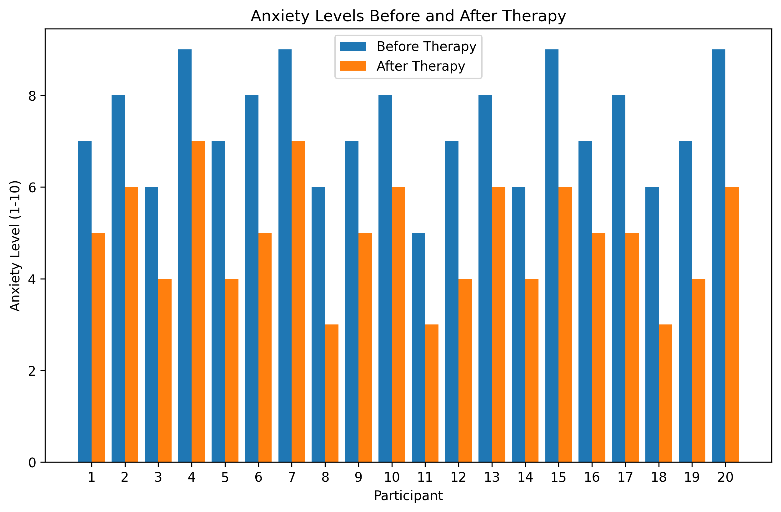
Let’s consider a simple example. Imagine you’re curious about whether a new therapy technique helps reduce anxiety. You might measure anxiety levels (perhaps on a scale from 1-10) before and after therapy for a group of 20 people.

Mathematics helps you answer questions like:

• Did anxiety decrease on average?

• How much did it decrease?

• Is the decrease large enough to be meaningful?

• Would we expect similar results with other people?

Let’s simulate this with a simple Python example:

import warnings
warnings.filterwarnings("ignore")
import matplotlib.pyplot as plt
plt.rcParams['axes.grid'] = False  # Ensure grid is turned off
plt.rcParams['figure.dpi'] = 300  # High resolution figures

# We'll use Python to help visualize and understand mathematical concepts
import numpy as np
import matplotlib.pyplot as plt

# Let's create some simulated data
# Anxiety scores before therapy (rating from 1-10)
before_therapy = [7, 8, 6, 9, 7, 8, 9, 6, 7, 8, 5, 7, 8, 6, 9, 7, 8, 6, 7, 9]

# Anxiety scores after therapy
after_therapy = [5, 6, 4, 7, 4, 5, 7, 3, 5, 6, 3, 4, 6, 4, 6, 5, 5, 3, 4, 6]

# Calculate the average (mean) score before and after
average_before = sum(before_therapy) / len(before_therapy)
average_after = sum(after_therapy) / len(after_therapy)

print(f"Average anxiety before therapy: {average_before}")
print(f"Average anxiety after therapy: {average_after}")
print(f"Average decrease in anxiety: {average_before - average_after}")

Average anxiety before therapy: 7.35
Average anxiety after therapy: 4.9
Average decrease in anxiety: 2.4499999999999993

Even in this simple example, we’re using mathematics! We calculated averages by adding up all the scores and dividing by the count of scores. This is called the arithmetic mean, which is a basic statistical concept.

The formula for the mean is: $\(\bar{x} = \frac{\sum_{i=1}^{n} x_i}{n}\)$

Don’t worry if this formula looks intimidating. It simply means:

• Add up all your values (that’s what \(\sum\) means)

• Divide by how many values you have (that’s \(n\))

Let’s visualize our therapy results:

# Create a simple before/after visualization
plt.figure(figsize=(10, 6))

# Create positions for the bars
bar_positions = np.arange(len(before_therapy))

# Create the bars
plt.bar(bar_positions - 0.2, before_therapy, width=0.4, label='Before Therapy')
plt.bar(bar_positions + 0.2, after_therapy, width=0.4, label='After Therapy')

# Add labels and title
plt.xlabel('Participant')
plt.ylabel('Anxiety Level (1-10)')
plt.title('Anxiety Levels Before and After Therapy')
plt.xticks(bar_positions, [str(i+1) for i in range(len(before_therapy))])
plt.legend()

# Show the plot
plt.show()

Mathematical Thinking vs. Calculation

An important distinction to make early on is between mathematical thinking and calculation.

Calculation is about following procedures to compute specific values. For example, adding up scores or multiplying numbers.

Mathematical thinking is much broader. It involves:

• Recognizing patterns

• Making logical connections

• Understanding relationships between quantities

• Asking “what if” questions

• Finding abstract structures in concrete situations

While computers (and calculators) are excellent at calculation, they need humans for mathematical thinking. This book aims to develop your mathematical thinking, not just your calculation skills.

The Power of Variables

One of the first steps in mathematical thinking is to use variables - symbols that can represent different values. In psychology, we might use variables like:

• \(A\) for anxiety level

• \(M\) for memory performance

• \(T\) for reaction time

Variables let us talk about general patterns rather than specific cases. For example, instead of saying “if someone’s anxiety decreases, their sleep quality might improve,” we could write:

If \(A\) decreases, then \(S\) might increase.

Where \(A\) is anxiety and \(S\) is sleep quality. This more precise language helps us build and test psychological theories.

Let’s look at a simple Python example using variables to model a relationship between study time and test performance:

# Let's create a simple model of how study time might relate to test scores

# Study time in hours (this is our independent variable)
study_time = [0, 1, 2, 3, 4, 5, 6, 7, 8]

# Test scores (dependent variable) - let's imagine there's a relationship
# but also some random variation (which is realistic)
np.random.seed(42)  # for reproducibility
base_score = 60  # starting score without studying
improvement_per_hour = 5  # each hour improves score by 5 points on average
random_variation = np.random.normal(0, 3, len(study_time))  # some random noise

# Calculate test scores based on our model
test_scores = [base_score + (improvement_per_hour * hours) + random_variation[i] 
              for i, hours in enumerate(study_time)]

# Make sure scores don't exceed 100
test_scores = [min(score, 100) for score in test_scores]

# Visualize the relationship
plt.figure(figsize=(10, 6))
plt.scatter(study_time, test_scores)
plt.xlabel('Study Time (hours)')
plt.ylabel('Test Score')
plt.title('Relationship Between Study Time and Test Performance')
plt.grid(True, linestyle='--', alpha=0.7)
plt.show()

# We could express this relationship using a simple mathematical model:
# Score = BaseScore + (ImprovementRate × StudyTime) + RandomVariation
# or using variables:
# S = B + (I × T) + R

print("Our mathematical model is: Score = 60 + (5 × StudyTime) + RandomVariation")

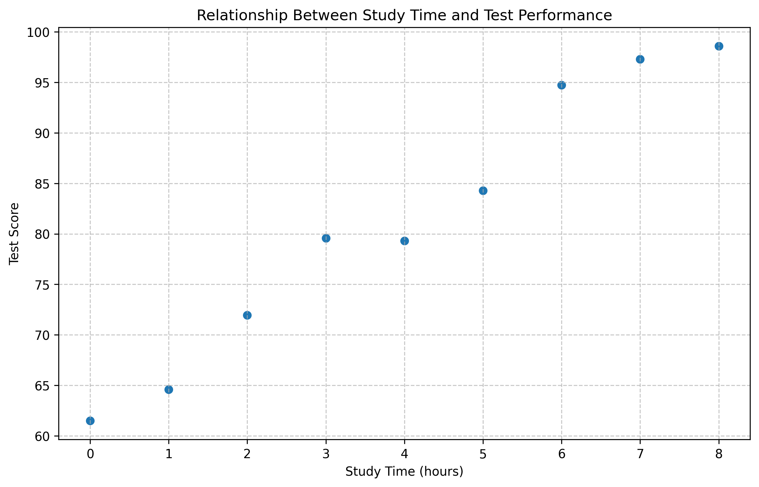
Our mathematical model is: Score = 60 + (5 × StudyTime) + RandomVariation

Patterns and Relationships

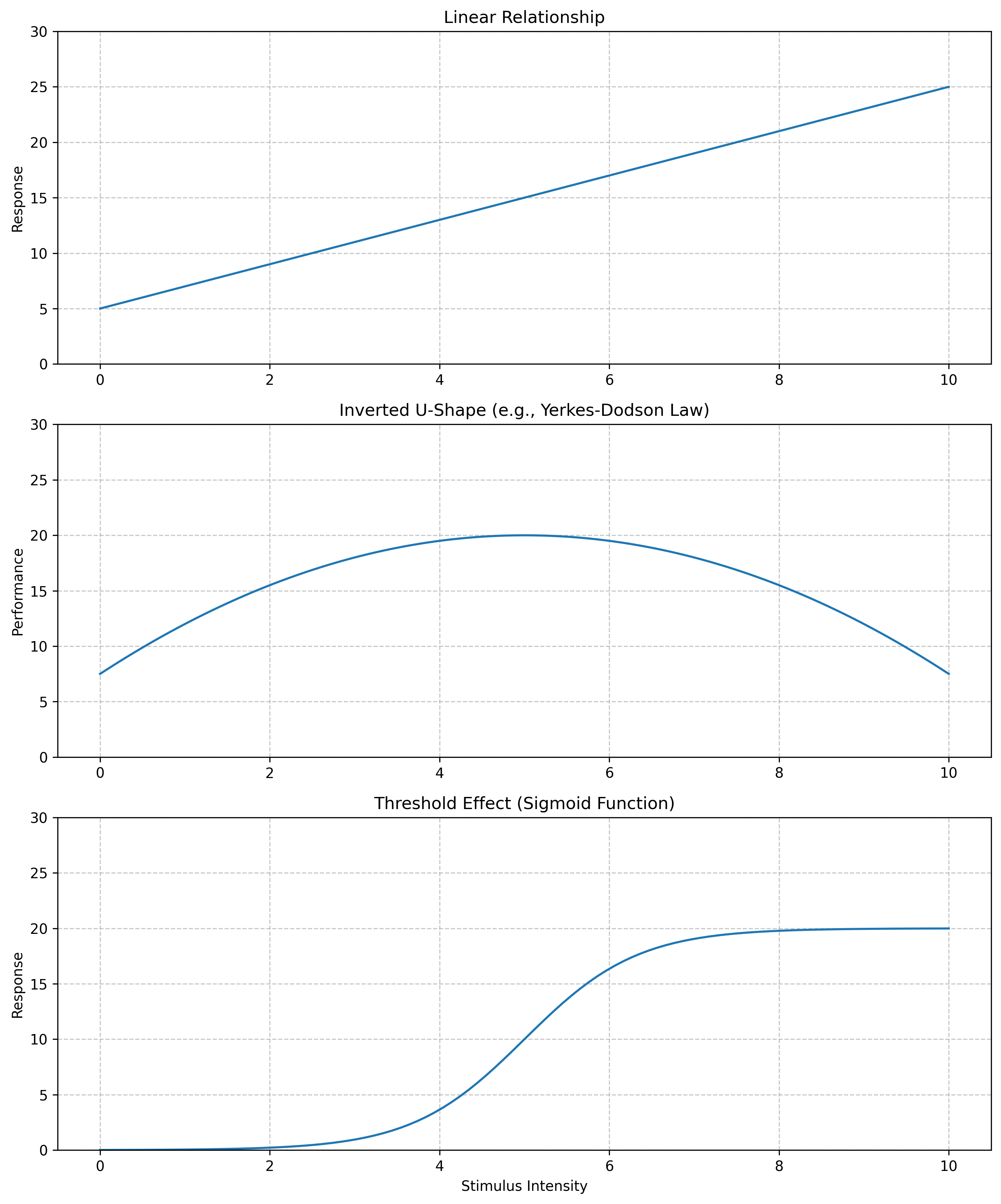
Mathematics helps us discover and describe patterns and relationships. In psychology, there are many interesting patterns:

1. Linear relationships: As one variable increases, another increases (or decreases) at a constant rate.

   • Example: As social media use increases, sleep quality might decrease linearly.

2. Non-linear relationships: Changes in one variable affect another, but not at a constant rate.

   • Example: The Yerkes-Dodson law suggests performance increases with arousal up to a point, then decreases (an inverted U-shape).

3. Threshold effects: Nothing happens until a certain value is reached, then change occurs.

   • Example: A person might not react to a stimulus until it reaches a certain intensity.

Let’s visualize some of these relationship types:

# Create data for different types of relationships
x = np.linspace(0, 10, 100)  # Create 100 points from 0 to 10

# Linear relationship (y = mx + b)
linear = 2*x + 5

# Quadratic relationship (inverted U-shape like Yerkes-Dodson)
quadratic = -0.5*(x-5)**2 + 20

# Threshold effect (sigmoid function)
threshold = 20 / (1 + np.exp(-1.5*(x-5)))

# Create a figure with three subplots
fig, axs = plt.subplots(3, 1, figsize=(10, 12))

# Plot each relationship
axs[0].plot(x, linear)
axs[0].set_title('Linear Relationship')
axs[0].set_ylabel('Response')
axs[0].grid(True, linestyle='--', alpha=0.7)
axs[0].set_ylim(0, 30)

axs[1].plot(x, quadratic)
axs[1].set_title('Inverted U-Shape (e.g., Yerkes-Dodson Law)')
axs[1].set_ylabel('Performance')
axs[1].grid(True, linestyle='--', alpha=0.7)
axs[1].set_ylim(0, 30)

axs[2].plot(x, threshold)
axs[2].set_title('Threshold Effect (Sigmoid Function)')
axs[2].set_xlabel('Stimulus Intensity')
axs[2].set_ylabel('Response')
axs[2].grid(True, linestyle='--', alpha=0.7)
axs[2].set_ylim(0, 30)

plt.tight_layout()
plt.show()

The Beauty of Mathematical Notation

Mathematical notation can seem intimidating at first, but it’s actually a powerful shorthand that helps us express complex ideas clearly and precisely.

For example, instead of saying “the average of all the values,” we can write:

\[\bar{x} = \frac{1}{n}\sum_{i=1}^{n} x_i\]

This might look complicated, but it’s just saying:

• Take each value (\(x_i\))

• Add them all up (that’s what \(\sum\) means)

• Divide by how many values you have (\(n\))

In psychology, we use mathematical notation to describe experiments, analyze data, and build theories. Don’t worry - we’ll introduce notation gradually throughout this book, always explaining what it means in plain language.

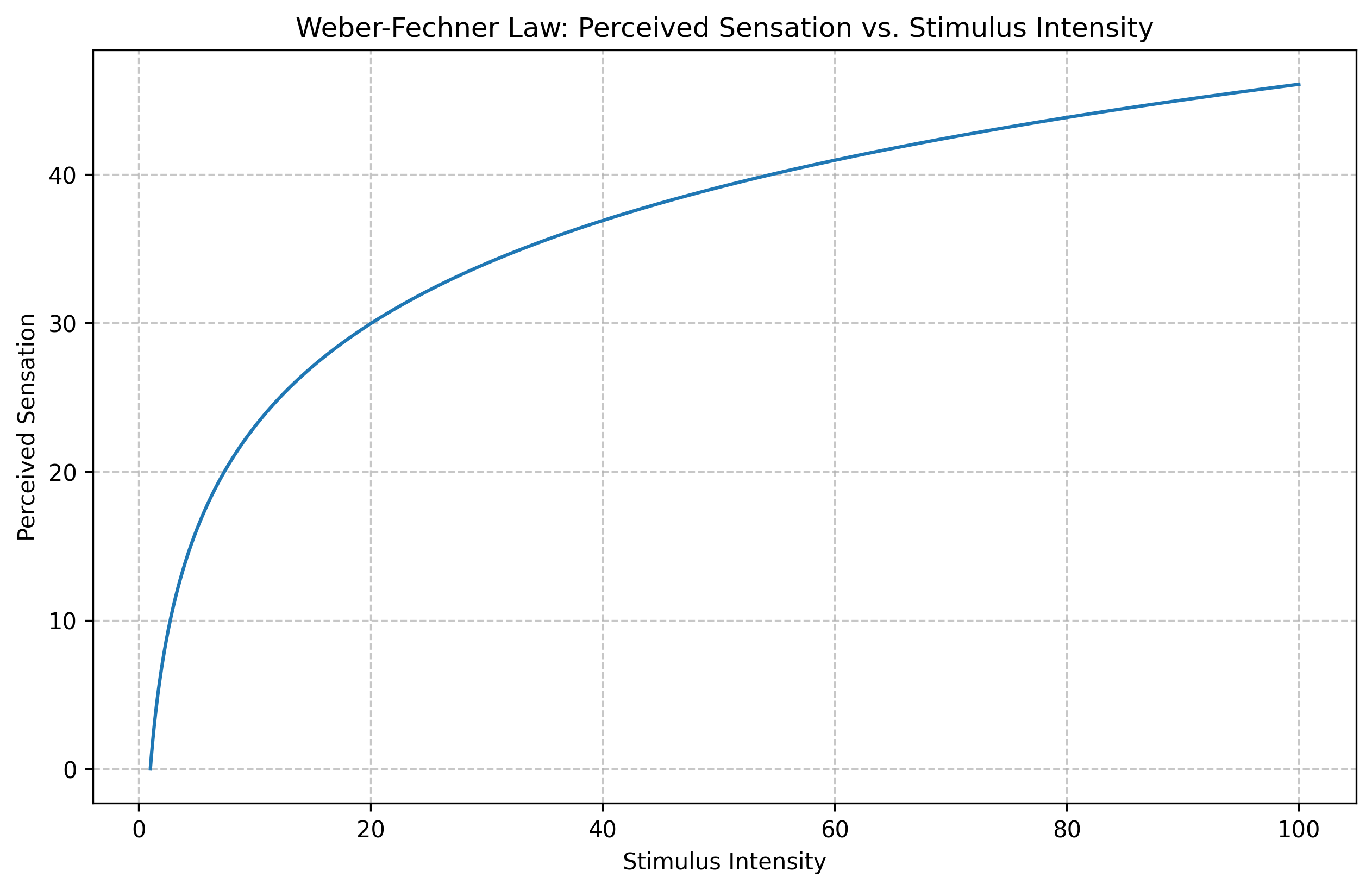
A Psychological Example: The Weber-Fechner Law

Let’s look at a real example from psychology: the Weber-Fechner Law. This law describes how we perceive changes in stimuli (like sounds, weights, or lights).

The basic idea is that we notice changes based on the relative difference, not the absolute difference. For example:

• Adding 1 gram to a 10-gram weight is noticeable (10% increase)

• Adding 1 gram to a 100-gram weight is barely noticeable (1% increase)

The mathematical formulation of the Weber-Fechner Law is:

\[S = k \ln\left(\frac{I}{I_0}\right)\]

Where:

• \(S\) is the perceived sensation

• \(I\) is the stimulus intensity

• \(I_0\) is the threshold intensity (minimum detectable)

• \(k\) is a constant

• \(\ln\) is the natural logarithm

This may look complex, but it expresses a simple idea: our perception scales logarithmically with stimulus intensity. Let’s see what this looks like:

# Visualize the Weber-Fechner Law
stimulus_intensity = np.linspace(1, 100, 1000)  # Range of stimulus intensities
threshold = 1  # Minimum detectable intensity
k = 10  # Constant

# Calculate perceived sensation according to Weber-Fechner Law
perceived_sensation = k * np.log(stimulus_intensity / threshold)

plt.figure(figsize=(10, 6))
plt.plot(stimulus_intensity, perceived_sensation)
plt.xlabel('Stimulus Intensity')
plt.ylabel('Perceived Sensation')
plt.title('Weber-Fechner Law: Perceived Sensation vs. Stimulus Intensity')
plt.grid(True, linestyle='--', alpha=0.7)
plt.show()

# Let's calculate some specific examples
def perceived_change(initial_intensity, new_intensity, k=10, threshold=1):
    """Calculate the change in perceived sensation based on Weber-Fechner Law"""
    initial_sensation = k * np.log(initial_intensity / threshold)
    new_sensation = k * np.log(new_intensity / threshold)
    return new_sensation - initial_sensation

# Example 1: Adding 1 unit to 10 units
change1 = perceived_change(10, 11)
print(f"Perceived change when adding 1 unit to 10 units: {change1:.4f}")

# Example 2: Adding 1 unit to 100 units
change2 = perceived_change(100, 101)
print(f"Perceived change when adding 1 unit to 100 units: {change2:.4f}")

# Example 3: Adding 10 units to 100 units
change3 = perceived_change(100, 110)
print(f"Perceived change when adding 10 units to 100 units: {change3:.4f}")

Perceived change when adding 1 unit to 10 units: 0.9531
Perceived change when adding 1 unit to 100 units: 0.0995
Perceived change when adding 10 units to 100 units: 0.9531

Key Takeaways from Chapter 1

In this introductory chapter, we’ve explored:

1. Why mathematics matters in psychology: It helps us measure, analyze, and understand human behavior.

2. Mathematical thinking vs. calculation: It’s about patterns and relationships, not just numbers.

3. Variables: Symbols that represent quantities and help us explore relationships.

4. Different types of relationships: Linear, non-linear, and threshold effects.

5. Mathematical notation: A powerful language for expressing ideas precisely.

6. Real psychological application: The Weber-Fechner Law, which describes how we perceive stimulus intensity.

Don’t worry if some concepts seemed challenging—this is just the beginning of our journey. Each chapter will build on this foundation, gradually introducing new ideas and showing how they apply to real psychological questions.

Practice Exercises

1. Reflection: Think about an area of psychology that interests you. What mathematical questions might arise in that area? For example, if you’re interested in cognitive psychology, you might wonder how to measure memory capacity or reaction times.

2. Basic Calculation: Calculate the average (mean) of these reaction times: 250ms, 275ms, 225ms, 300ms, 265ms.

3. Pattern Recognition: Look at this sequence: 2, 4, 8, 16, … What might the next number be? What pattern do you see?

4. Python Practice: Modify the therapy example code to calculate the median anxiety scores (the middle value when sorted) instead of the mean. How do the results compare?

5. Application: Think of a real-life situation where the Weber-Fechner Law might apply. For example, why might a \(5 price increase seem significant for a \)20 item but negligible for a $200 item?

In the next chapter, we’ll explore number systems and basic operations, building a stronger foundation for your mathematical journey.