Chapter 2: Number Systems and Basic Operations#
Mathematics for Psychologists and Computation
Welcome to Chapter 2! In this chapter, we’ll explore the foundations of mathematics: numbers and the basic operations we perform with them. These concepts might seem simple, but they form the building blocks for everything else we’ll learn in this book.
Remember, we’re starting from the very beginning, so don’t worry if some of this feels like review. A solid foundation is essential for the more complex ideas we’ll explore later.
import warnings
warnings.filterwarnings("ignore")
import matplotlib.pyplot as plt
plt.rcParams['axes.grid'] = False  # Ensure grid is turned off
plt.rcParams['figure.dpi'] = 300  # High resolution figures
Types of Numbers#
Let’s start by understanding the different types of numbers we’ll encounter:
Natural Numbers#
Natural numbers are the counting numbers we learn first as children: 1, 2, 3, 4, 5, …
We use natural numbers to count distinct objects. For example, in psychology, you might count:
Number of participants in a study
Number of correct responses on a test
Number of sessions in a therapy program
Whole Numbers#
Whole numbers include all natural numbers plus zero: 0, 1, 2, 3, 4, …
Zero is important! In psychology, zero might represent:
No responses on a particular question
Baseline or starting point on a scale
Absence of a particular behavior
# Let's create some examples of natural and whole numbers in Python
import numpy as np
import matplotlib.pyplot as plt
# Natural numbers - positive integers used for counting
natural_numbers = [1, 2, 3, 4, 5, 6, 7, 8, 9, 10]
print("Natural numbers (for counting):", natural_numbers)
# Whole numbers - natural numbers plus zero
whole_numbers = [0, 1, 2, 3, 4, 5, 6, 7, 8, 9, 10]
print("Whole numbers (including zero):", whole_numbers)
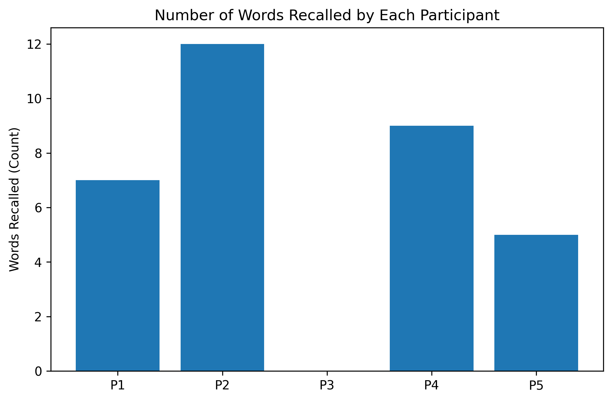
# A psychology example: response counts in a memory experiment
participants = ['P1', 'P2', 'P3', 'P4', 'P5']
recalled_words = [7, 12, 0, 9, 5] # Note: zero is valid here (no words recalled)
plt.figure(figsize=(8, 5))
plt.bar(participants, recalled_words)
plt.title('Number of Words Recalled by Each Participant')
plt.ylabel('Words Recalled (Count)')
plt.show()
Natural numbers (for counting): [1, 2, 3, 4, 5, 6, 7, 8, 9, 10]
Whole numbers (including zero): [0, 1, 2, 3, 4, 5, 6, 7, 8, 9, 10]
Division (÷)#
Division is the inverse of multiplication. When we divide \(a ÷ b\), we’re finding out how many times \(b\) goes into \(a\).
Key things to remember:
Not commutative: \(a ÷ b ≠ b ÷ a\) (order matters)
\(a ÷ 1 = a\) (dividing by 1 doesn’t change the value)
\(a ÷ a = 1\) (dividing a number by itself gives 1, if \(a ≠ 0\))
Division by zero is undefined
In psychology, division is used to:
Calculate averages (sum ÷ count)
Convert raw scores to percentages
Find rates (events per time period)
Normalize data
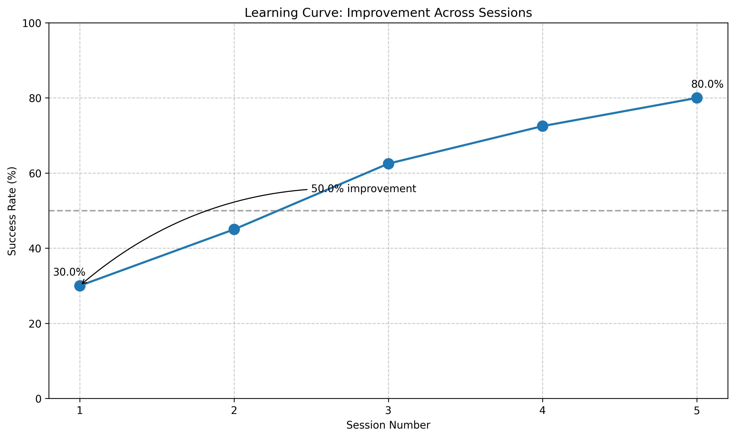
# Psychology example for division
# Let's look at response rates in a behavioral experiment

# Number of correct responses in a learning task across 5 sessions
sessions = [1, 2, 3, 4, 5]
correct_responses = [12, 18, 25, 29, 32]
total_trials = 40  # Each session had 40 trials

# Calculate success rates
success_rates = []
for responses in correct_responses:
    rate = responses / total_trials  # Division to get proportion
    success_rates.append(rate)

# Convert to percentages
percentages = [rate * 100 for rate in success_rates]

# Display results
print("Learning Progress Across Sessions:\n")
print(f"{'Session':<10} {'Correct':<10} {'Total':<10} {'Rate':<10} {'Percentage':<10}")
print("-" * 50)

for i, session in enumerate(sessions):
    print(f"{session:<10} {correct_responses[i]:<10} {total_trials:<10} {success_rates[i]:.2f}")

# Calculate learning improvement
first_session = success_rates[0]
last_session = success_rates[-1]
improvement = last_session - first_session
improvement_percent = improvement * 100

print(f"\nImprovement from first to last session: {improvement_percent:.1f}%")

# Visualize the learning curve
plt.figure(figsize=(10, 6))
plt.plot(sessions, percentages, marker='o', markersize=10, linewidth=2)
plt.axhline(y=50, color='gray', linestyle='--', alpha=0.7, label='Chance level (50%)')
plt.xlabel('Session Number')
plt.ylabel('Success Rate (%)')
plt.title('Learning Curve: Improvement Across Sessions')
plt.ylim(0, 100)
plt.grid(True, linestyle='--', alpha=0.7)
plt.xticks(sessions)

# Annotate the first and last points
plt.annotate(f"{percentages[0]:.1f}%", (sessions[0], percentages[0]),
             textcoords="offset points", xytext=(-10,10), ha='center')
plt.annotate(f"{percentages[-1]:.1f}%", (sessions[-1], percentages[-1]),
             textcoords="offset points", xytext=(10,10), ha='center')

# Add an arrow showing improvement
plt.annotate(f"{improvement_percent:.1f}% improvement",
             xy=(sessions[0], percentages[0]),
             xytext=(2.5, (percentages[0] + percentages[-1])/2),  # Changed to avoid duplicate xytext
             textcoords='data',
             arrowprops=dict(arrowstyle="->", connectionstyle="arc3,rad=.2"))

plt.tight_layout()
plt.show()
Learning Progress Across Sessions:

Session    Correct    Total      Rate       Percentage
--------------------------------------------------
1          12         40         0.30
2          18         40         0.45
3          25         40         0.62
4          29         40         0.72
5          32         40         0.80

Improvement from first to last session: 50.0%
Order of Operations#
When an expression contains multiple operations, we need to follow the correct order to get the right answer. The standard order is summarized by the acronym PEMDAS:
Parentheses - Calculate expressions inside parentheses first
Exponents - Calculate powers and roots
Multiplication and Division - Perform these from left to right
Addition and Subtraction - Perform these from left to right
This order ensures that everyone gets the same answer when calculating complex expressions.
# Examples of order of operations
example1 = 2 + 3 * 4
example2 = (2 + 3) * 4
example3 = 10 - 6 / 2 + 3
example4 = 3 ** 2 + 4 * 2

print(f"2 + 3 * 4 = {example1}")
print(f"(2 + 3) * 4 = {example2}")
print(f"10 - 6 / 2 + 3 = {example3}")
print(f"3 ** 2 + 4 * 2 = {example4}")

# Let's create a psychology example using order of operations
# Imagine a formula for predicting test anxiety from hours studied and prior performance

def anxiety_score(hours_studied, prior_performance, baseline=50):
    # A made-up formula for illustration
    # Anxiety = Baseline - (Hours_Studied * 2) + (10 - Prior_Performance) * 3
    # Higher prior performance (0-10) leads to lower anxiety
    # More hours studied generally reduces anxiety

    return baseline - (hours_studied * 2) + (10 - prior_performance) * 3

# Try with some example values
student1 = anxiety_score(hours_studied=5, prior_performance=8)
student2 = anxiety_score(hours_studied=2, prior_performance=4)
student3 = anxiety_score(hours_studied=10, prior_performance=6)

print("\nTest Anxiety Predictions:")
print(f"Student 1 (5 hours, 8/10 prior): {student1}")
print(f"Student 2 (2 hours, 4/10 prior): {student2}")
print(f"Student 3 (10 hours, 6/10 prior): {student3}")

# Step by step breakdown for student 1
print("\nStep-by-step calculation for Student 1:")
print("anxiety = 50 - (5 * 2) + (10 - 8) * 3")
print("       = 50 - 10 + 2 * 3")
print("       = 50 - 10 + 6")
print("       = 40 + 6")
print("       = 46")
2 + 3 * 4 = 14
(2 + 3) * 4 = 20
10 - 6 / 2 + 3 = 10.0
3 ** 2 + 4 * 2 = 17

Test Anxiety Predictions:
Student 1 (5 hours, 8/10 prior): 46
Student 2 (2 hours, 4/10 prior): 64
Student 3 (10 hours, 6/10 prior): 42

Step-by-step calculation for Student 1:
anxiety = 50 - (5 * 2) + (10 - 8) * 3
       = 50 - 10 + 2 * 3
       = 50 - 10 + 6
       = 40 + 6
       = 46
Working with Large and Small Numbers#
In psychology research, we often encounter very large numbers (like the population of a country) or very small numbers (like precise reaction times in milliseconds). Scientific notation helps us work with these numbers efficiently.
Scientific notation expresses a number as a product of a coefficient and a power of 10:
\(a \times 10^b\)
Where \(a\) is a number between 1 and 10, and \(b\) is an integer.
Examples:
5,280 = \(5.28 \times 10^3\)
0.000072 = \(7.2 \times 10^{-5}\)
# Examples of scientific notation in psychology
import math

# Some examples of large and small numbers in psychology
neurons_in_brain = 86000000000  # 86 billion neurons in the human brain
synapse_distance = 0.000000020  # 20 nanometers (average distance across a synapse)
action_potential = 0.001  # 1 millisecond (typical duration of a neural action potential)
us_population = 331000000  # 331 million (approximate US population)

# Convert to scientific notation
def to_scientific(num):
    exponent = math.floor(math.log10(abs(num)))
    coefficient = num / (10 ** exponent)
    return coefficient, exponent

# Display the numbers in standard and scientific notation
print("Large and Small Numbers in Psychology\n")

numbers = {
    "Neurons in human brain": neurons_in_brain,
    "Synapse distance (m)": synapse_distance,
    "Action potential duration (s)": action_potential,
    "US population": us_population
}

for label, num in numbers.items():
    coef, exp = to_scientific(num)
    print(f"{label}:")
    print(f"  Standard notation: {num}")
    print(f"  Scientific notation: {coef:.2f} × 10^{exp}\n")

# In Python, we can use 'e' notation for scientific notation
print("Using Python's scientific notation:")
print(f"Neurons in brain: {neurons_in_brain:.2e}")
print(f"Synapse distance: {synapse_distance:.2e}")
Large and Small Numbers in Psychology

Neurons in human brain:
  Standard notation: 86000000000
  Scientific notation: 8.60 × 10^10

Synapse distance (m):
  Standard notation: 2e-08
  Scientific notation: 2.00 × 10^-8

Action potential duration (s):
  Standard notation: 0.001
  Scientific notation: 1.00 × 10^-3

US population:
  Standard notation: 331000000
  Scientific notation: 3.31 × 10^8

Using Python's scientific notation:
Neurons in brain: 8.60e+10
Synapse distance: 2.00e-08
Numbers in Psychological Research#
Let’s conclude this chapter by looking at how number systems and operations appear in psychological research.
Measurement scales: Psychology uses different types of scales for measuring variables:
Nominal scales use numbers as labels (e.g., 1=male, 2=female)
Ordinal scales rank items but don’t specify exact differences (e.g., 1st, 2nd, 3rd place)
Interval scales have equal intervals but no absolute zero (e.g., temperature in Celsius)
Ratio scales have equal intervals and an absolute zero (e.g., reaction time)
Descriptive statistics: We use numbers to summarize data:
Central tendency (mean, median, mode)
Variability (range, standard deviation)
Proportions and percentages
Experimental design: Numbers help us design studies:
Sample size calculations
Random assignment to conditions
Counterbalancing procedures
# Example of different measurement scales in psychology
import pandas as pd
from IPython.display import display, HTML
# Create sample data with different types of variables
data = {
'Participant': [1, 2, 3, 4, 5],
'Gender': ['Male', 'Female', 'Non-binary', 'Female', 'Male'], # Nominal
'Education': ['High School', 'Bachelor', 'Master', 'PhD', 'Bachelor'], # Nominal
'Satisfaction': [3, 5, 2, 4, 3], # Ordinal (1-5 scale)
'Age': [24, 32, 45, 19, 56], # Ratio
'Response Time (ms)': [342, 287, 512, 298, 376], # Ratio
'IQ Score': [105, 118, 124, 110, 95] # Interval
}
# Create a DataFrame
df = pd.DataFrame(data)
# Display the data
print("Sample Psychological Data with Different Measurement Scales:\n")
display(df)
# Calculate some basic statistics
# We'll exclude the nominal variables (Gender, Education) from these calculations
numeric_vars = ['Satisfaction', 'Age', 'Response Time (ms)', 'IQ Score']
numeric_df = df[numeric_vars]
# Calculate statistics
means = numeric_df.mean()
medians = numeric_df.median()
std_devs = numeric_df.std()
minimums = numeric_df.min()
maximums = numeric_df.max()
ranges = maximums - minimums
# Create a summary statistics DataFrame
stats_df = pd.DataFrame({
'Mean': means,
'Median': medians,
'Std Dev': std_devs,
'Min': minimums,
'Max': maximums,
'Range': ranges
})
print("\nSummary Statistics:\n")
display(stats_df)
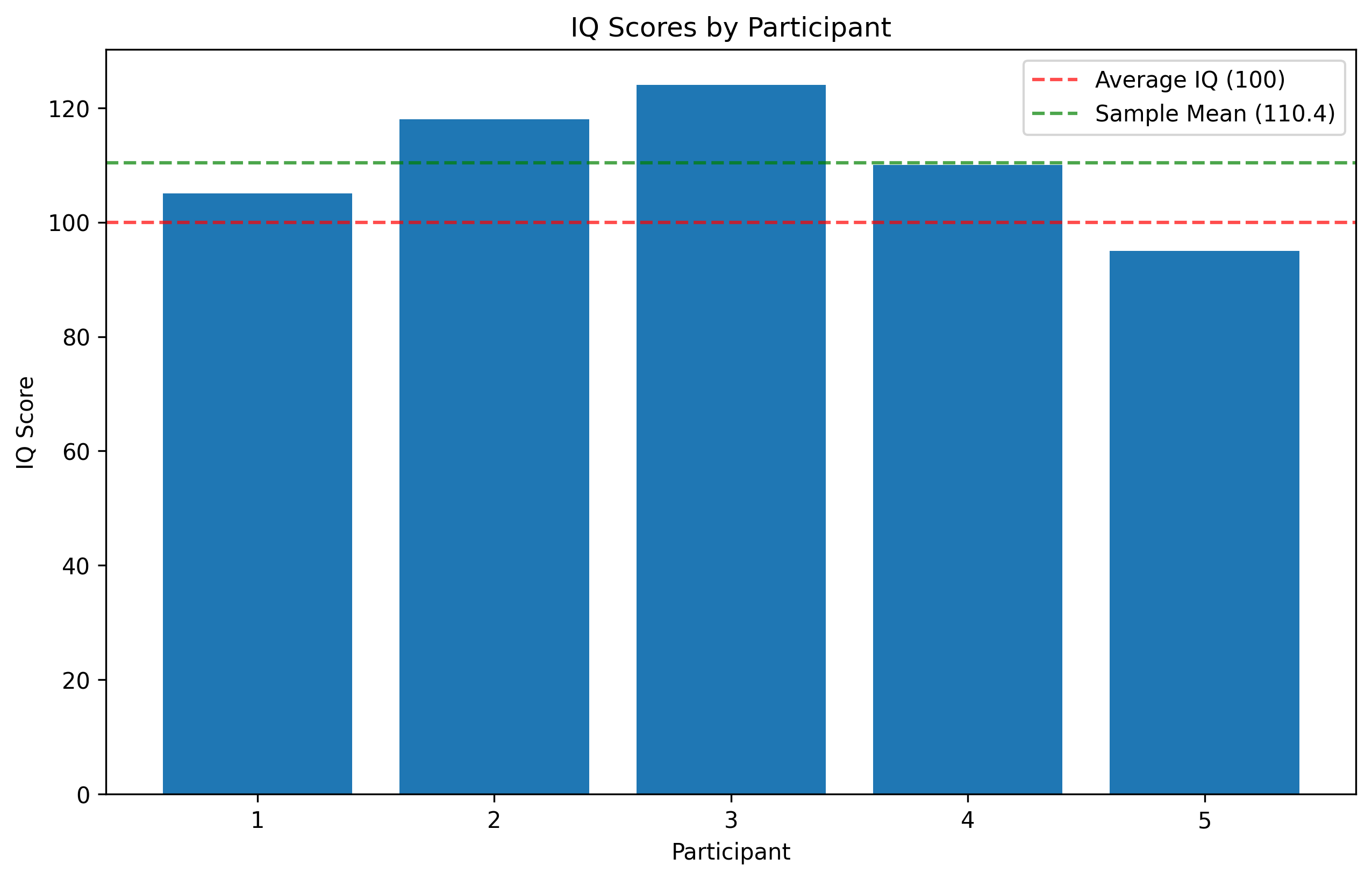
# Visualize one of the variables
plt.figure(figsize=(10, 6))
plt.bar(df['Participant'], df['IQ Score'])
plt.axhline(y=100, color='red', linestyle='--', alpha=0.7, label='Average IQ (100)')
plt.axhline(y=stats_df.loc['IQ Score', 'Mean'], color='green', linestyle='--',
alpha=0.7, label=f'Sample Mean ({stats_df.loc["IQ Score", "Mean"]:.1f})')
plt.xlabel('Participant')
plt.ylabel('IQ Score')
plt.title('IQ Scores by Participant')
plt.legend()
plt.show()
Sample Psychological Data with Different Measurement Scales:
| Participant | Gender | Education | Satisfaction | Age | Response Time (ms) | IQ Score | |
|---|---|---|---|---|---|---|---|
| 0 | 1 | Male | High School | 3 | 24 | 342 | 105 |
| 1 | 2 | Female | Bachelor | 5 | 32 | 287 | 118 |
| 2 | 3 | Non-binary | Master | 2 | 45 | 512 | 124 |
| 3 | 4 | Female | PhD | 4 | 19 | 298 | 110 |
| 4 | 5 | Male | Bachelor | 3 | 56 | 376 | 95 |
Summary Statistics:
| Mean | Median | Std Dev | Min | Max | Range | |
|---|---|---|---|---|---|---|
| Satisfaction | 3.4 | 3.0 | 1.140175 | 2 | 5 | 3 |
| Age | 35.2 | 32.0 | 15.221695 | 19 | 56 | 37 |
| Response Time (ms) | 363.0 | 342.0 | 90.570415 | 287 | 512 | 225 |
| IQ Score | 110.4 | 110.0 | 11.282730 | 95 | 124 | 29 |
Key Takeaways from Chapter 2#
In this chapter, we’ve explored:
Different types of numbers:
Natural numbers (counting numbers: 1, 2, 3, …)
Whole numbers (natural numbers plus zero: 0, 1, 2, …)
Integers (whole numbers and their negatives: …, -2, -1, 0, 1, 2, …)
Rational numbers (fractions or ratios of integers)
Irrational numbers (non-repeating, non-terminating decimals like π)
Real numbers (all rational and irrational numbers)
The number line as a visual representation of numbers
Basic operations:
Addition (combining quantities)
Subtraction (finding differences)
Multiplication (repeated addition)
Division (partitioning or finding ratios)
Order of operations (PEMDAS) for solving complex expressions
Scientific notation for working with very large or small numbers
Applications in psychology including measurement scales and descriptive statistics
Understanding these fundamentals will help you as we progress to more advanced topics. In the next chapter, we’ll dive into fractions and decimals, essential concepts for understanding proportions and precise measurements in psychological research.
Practice Exercises#
Number Classification: Identify which type(s) of numbers these are:
0
-7
3.25
√9
π
Basic Operations: Calculate these expressions and explain which operations you performed first and why:
8 + 4 × 3
(8 + 4) × 3
16 - 8 ÷ 4 + 2
3² + 10 ÷ 2
Psychological Application: A researcher measures anxiety before and after treatment for 6 participants. The scores (on a 0-10 scale) are:
Before: [8, 7, 9, 6, 10, 8]
After: [5, 6, 8, 3, 7, 6]
Calculate:
The average (mean) anxiety before and after treatment
The change in anxiety for each participant
The average (mean) change across all participants
Scientific Notation: Convert these psychology-related numbers to scientific notation:
Human population: 8,000,000,000
Dopamine molecule size: 0.000000001 meters
Typical reaction time: 0.25 seconds
Python Practice: Modify the weighted scoring example to incorporate a new “Social Skills” factor with a raw score of 40 and a weight of 1.5. Recalculate the total weighted score.
Challenge Question: A psychology experiment has 24 participants. The researcher wants to divide them equally into 4 experimental conditions. How many participants will be in each condition? If each condition requires 2 hours of testing per participant, how many total hours will the experiment take?
Integers#
Integers include all whole numbers and their negative counterparts: …, -3, -2, -1, 0, 1, 2, 3, …
In psychology, negative integers might represent:
Below-average scores (when zero is the average)
Decreases in behavior or performance
Positions on a bipolar scale (e.g., strongly disagree [-2] to strongly agree [+2])
# Example of integers in psychology
# Let's imagine a mood rating scale from -5 (very negative) to +5 (very positive)

days = ['Monday', 'Tuesday', 'Wednesday', 'Thursday', 'Friday', 'Saturday', 'Sunday']
mood_ratings = [-2, 0, 1, -1, 3, 4, 2]  # Notice both positive and negative integers

plt.figure(figsize=(10, 6))
bars = plt.bar(days, mood_ratings)

# Color the bars based on positive or negative values
for i, bar in enumerate(bars):
    if mood_ratings[i] < 0:
        bar.set_color('salmon')
    else:
        bar.set_color('skyblue')

plt.axhline(y=0, color='gray', linestyle='-', alpha=0.3)  # Add a line at zero
plt.title('Daily Mood Ratings')
plt.ylabel('Mood (-5 to +5 scale)')
plt.ylim(-5, 5)  # Set the y-axis limits
plt.show()

# Calculate the average mood
average_mood = sum(mood_ratings) / len(mood_ratings)
print(f"Average mood for the week: {average_mood}")
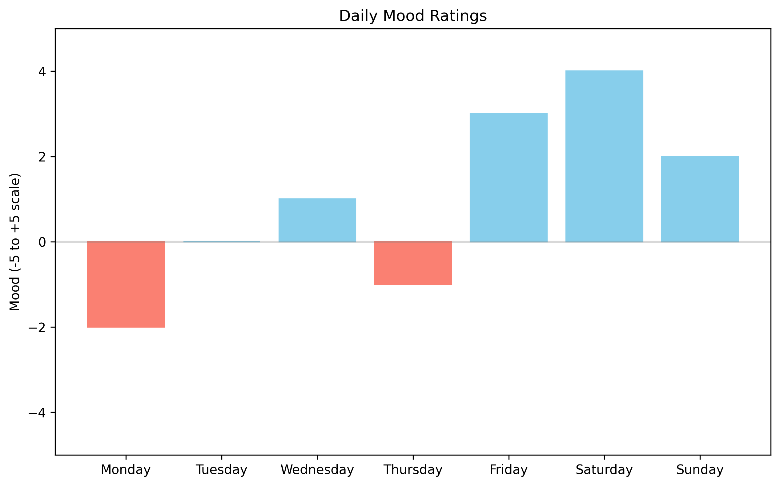
Average mood for the week: 1.0
Rational Numbers#
Rational numbers are fractions or ratios of integers. They can be expressed as \(\frac{p}{q}\) where \(p\) and \(q\) are integers and \(q \neq 0\).
Examples: \(\frac{1}{2}\), \(\frac{3}{4}\), \(-\frac{5}{3}\), 0.75, 2.5
In psychology, rational numbers appear frequently:
Test scores (75% or 0.75 correct)
Proportions (⅓ of participants responded in a certain way)
Precise measurements (reaction time of 0.357 seconds)
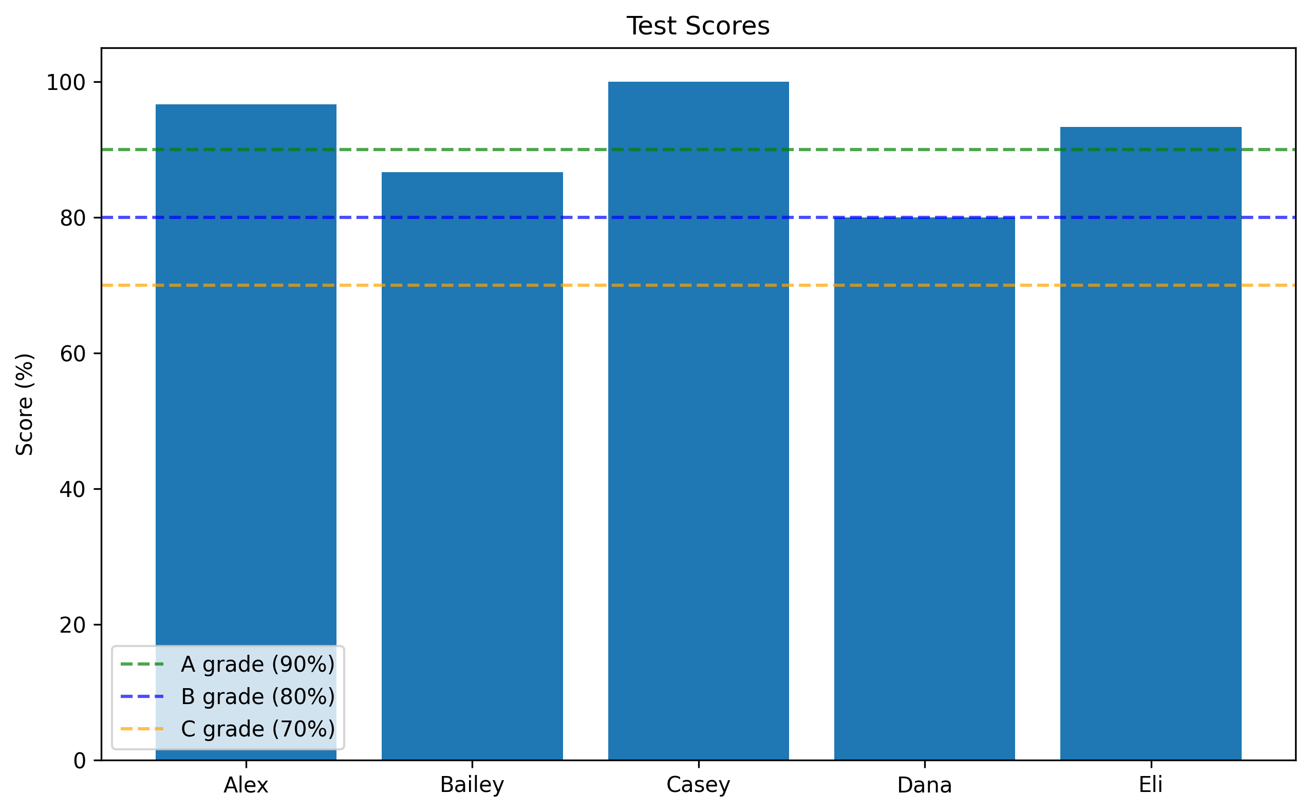
# Example of rational numbers in psychology
# Let's look at test scores as proportions

students = ['Alex', 'Bailey', 'Casey', 'Dana', 'Eli']
scores_as_fractions = [29/30, 26/30, 30/30, 24/30, 28/30]  # Fractions (rational numbers)
scores_as_percentages = [score * 100 for score in scores_as_fractions]  # Convert to percentages

# Display the scores in different formats
for i, student in enumerate(students):
    fraction = scores_as_fractions[i]
    decimal = float(fraction)  # Convert fraction to decimal
    percentage = scores_as_percentages[i]

    print(f"{student}:")
    print(f"  - As fraction: {int(fraction*30)}/30")
    print(f"  - As decimal: {decimal:.3f}")
    print(f"  - As percentage: {percentage:.1f}%\n")

# Visualize the scores
plt.figure(figsize=(10, 6))
plt.bar(students, scores_as_percentages)
plt.axhline(y=90, color='green', linestyle='--', alpha=0.7, label='A grade (90%)')
plt.axhline(y=80, color='blue', linestyle='--', alpha=0.7, label='B grade (80%)')
plt.axhline(y=70, color='orange', linestyle='--', alpha=0.7, label='C grade (70%)')
plt.title('Test Scores')
plt.ylabel('Score (%)')
plt.ylim(0, 105)  # Set y-axis limits
plt.legend()
plt.show()
Alex:
  - As fraction: 29/30
  - As decimal: 0.967
  - As percentage: 96.7%

Bailey:
  - As fraction: 26/30
  - As decimal: 0.867
  - As percentage: 86.7%

Casey:
  - As fraction: 30/30
  - As decimal: 1.000
  - As percentage: 100.0%

Dana:
  - As fraction: 24/30
  - As decimal: 0.800
  - As percentage: 80.0%

Eli:
  - As fraction: 28/30
  - As decimal: 0.933
  - As percentage: 93.3%
Irrational Numbers#
Irrational numbers cannot be expressed as fractions. They have decimal expansions that go on forever without repeating patterns.
Famous examples include:
\(\pi\) (pi) ≈ 3.14159…
\(e\) (Euler’s number) ≈ 2.71828…
\(\sqrt{2}\) (square root of 2) ≈ 1.41421…
In psychology, irrational numbers sometimes emerge in formulas and calculations, especially in advanced statistical methods.
# Let's explore some common irrational numbers
import math
# Some important irrational numbers
pi = math.pi
e = math.e
sqrt2 = math.sqrt(2)
print(f"π (pi) ≈ {pi}")
print(f"e (Euler's number) ≈ {e}")
print(f"√2 (square root of 2) ≈ {sqrt2}")
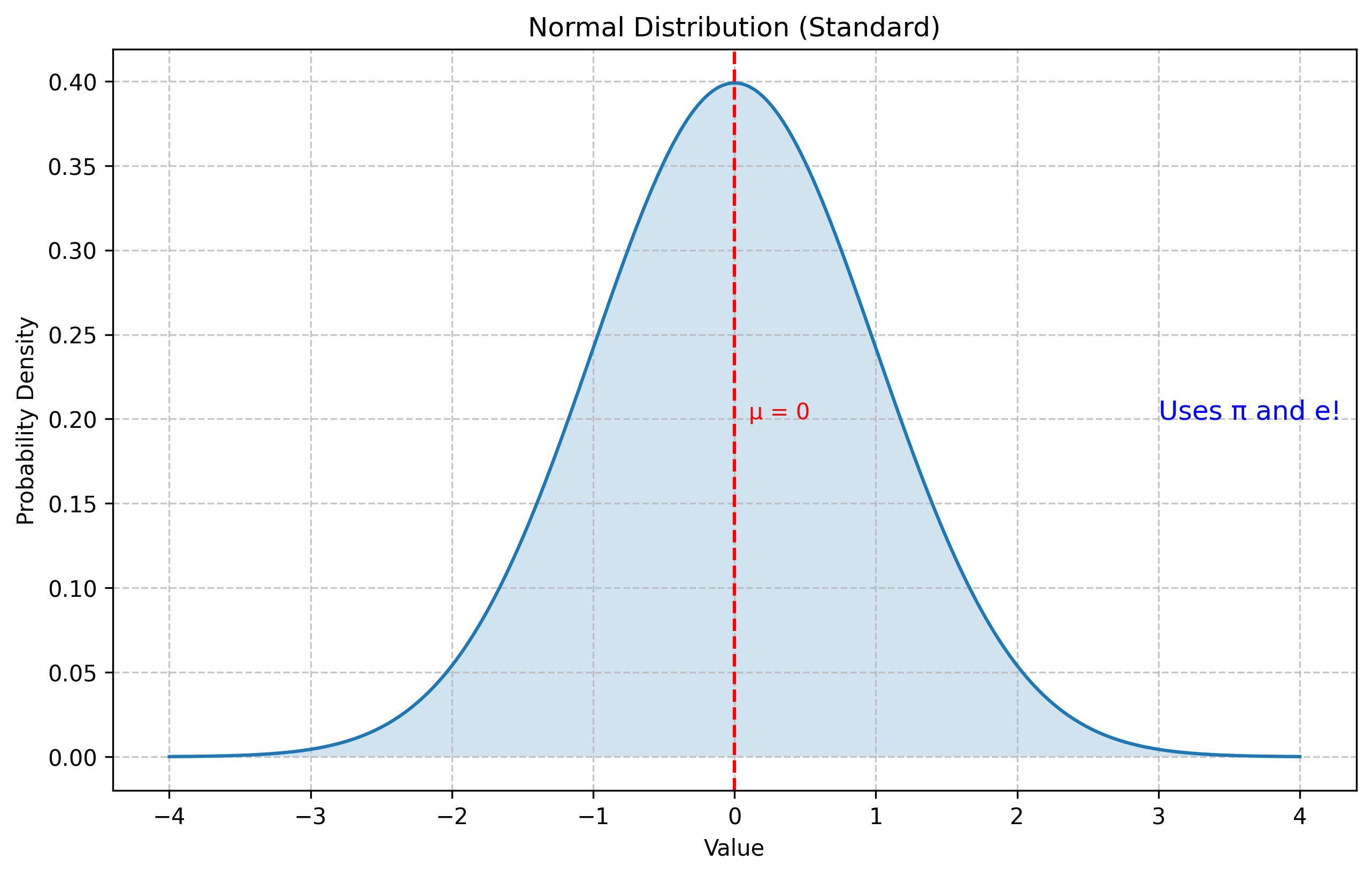
# In psychology, the normal distribution formula uses both π and e
# The formula for the normal distribution probability density function is:
# f(x) = (1 / (σ * √(2π))) * e^(-(x-μ)²/(2σ²))
# Let's visualize the normal distribution which is important in psychology
x = np.linspace(-4, 4, 1000) # Generate x values from -4 to 4
mean = 0 # μ (mu)
std_dev = 1 # σ (sigma)
# Calculate the normal distribution using the formula
normal_dist = (1 / (std_dev * np.sqrt(2 * pi))) * np.exp(-(x - mean)**2 / (2 * std_dev**2))
plt.figure(figsize=(10, 6))
plt.plot(x, normal_dist)
plt.title('Normal Distribution (Standard)')
plt.xlabel('Value')
plt.ylabel('Probability Density')
plt.grid(True, linestyle='--', alpha=0.7)
plt.axvline(x=mean, color='red', linestyle='--', label='Mean (μ)')
plt.text(mean+0.1, 0.2, 'μ = 0', color='red')
plt.text(3, 0.2, 'Uses π and e!', fontsize=12, color='blue')
plt.fill_between(x, normal_dist, 0, alpha=0.2) # Shade under the curve
plt.show()
print("\nThe normal distribution is crucial in psychology and statistics.")
print("It describes how many psychological variables are distributed in the population.")
print("Examples include IQ scores, personality traits, and reaction times (after transformation).")
π (pi) ≈ 3.141592653589793
e (Euler's number) ≈ 2.718281828459045
√2 (square root of 2) ≈ 1.4142135623730951
The normal distribution is crucial in psychology and statistics.
It describes how many psychological variables are distributed in the population.
Examples include IQ scores, personality traits, and reaction times (after transformation).
Real Numbers#
Real numbers include all rational and irrational numbers. They represent all possible points on a number line.
In psychology, real numbers are used for:
Continuous measurements (time, weight, height)
Statistical values (means, standard deviations)
Scale scores (personality inventories, mood ratings)
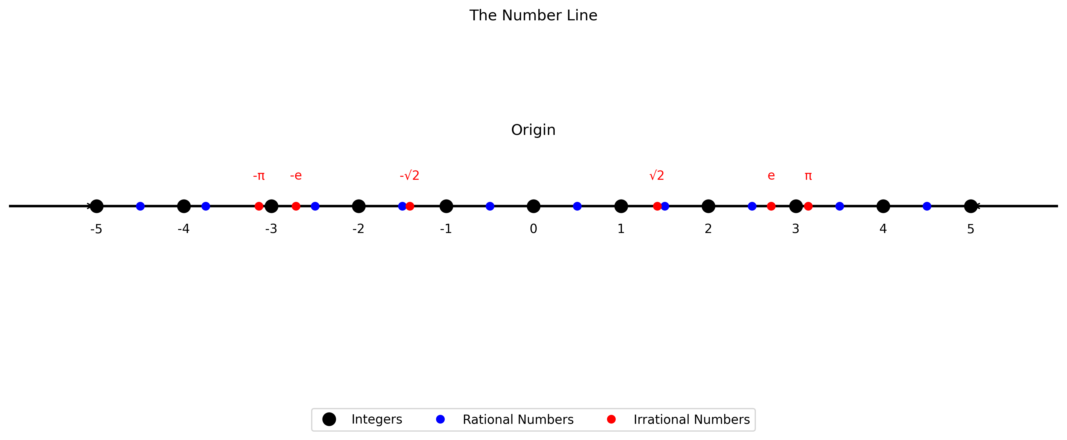
The Number Line#
The number line is a visual representation of real numbers. It’s a horizontal line with points corresponding to numbers, increasing from left to right.
Important features:
0 is usually at the center
Positive numbers are to the right of 0
Negative numbers are to the left of 0
Equal intervals represent equal differences between numbers
Let’s visualize the number line and explore different types of numbers on it:
# Let's visualize the number line with different types of numbers
plt.figure(figsize=(12, 5))

# Draw the number line
plt.axhline(y=0, color='black', linestyle='-', linewidth=2)

# Mark integers from -5 to 5
for i in range(-5, 6):
    plt.plot(i, 0, 'ko', markersize=10)  # 'ko' means black circle marker
    plt.text(i, -0.15, str(i), ha='center')

# Mark some rational numbers
rational_points = [-4.5, -3.75, -2.5, -1.5, -0.5, 0.5, 1.5, 2.5, 3.5, 4.5]
for point in rational_points:
    plt.plot(point, 0, 'bo', markersize=6)  # 'bo' means blue circle marker

# Mark some irrational numbers
irrational_points = [math.pi, -math.pi, math.e, -math.e, math.sqrt(2), -math.sqrt(2)]
irrational_labels = ['π', '-π', 'e', '-e', '√2', '-√2']

for i, point in enumerate(irrational_points):
    plt.plot(point, 0, 'ro', markersize=6)  # 'ro' means red circle marker
    plt.text(point, 0.15, irrational_labels[i], ha='center', color='red')

# Add some annotations
plt.text(0, 0.4, 'Origin', ha='center', fontsize=12)
plt.annotate('', xy=(5, 0), xytext=(5.5, 0), arrowprops=dict(arrowstyle="->"))
plt.annotate('', xy=(-5, 0), xytext=(-5.5, 0), arrowprops=dict(arrowstyle="->"))

# Set plot limits and remove axes
plt.xlim(-6, 6)
plt.ylim(-1, 1)
plt.axis('off')
plt.title('The Number Line')

# Add a legend
plt.plot([], [], 'ko', markersize=10, label='Integers')
plt.plot([], [], 'bo', markersize=6, label='Rational Numbers')
plt.plot([], [], 'ro', markersize=6, label='Irrational Numbers')
plt.legend(loc='upper center', bbox_to_anchor=(0.5, -0.05), ncol=3)

plt.tight_layout()
plt.show()
Basic Operations with Numbers#
Now let’s review the four basic operations: addition, subtraction, multiplication, and division. These form the foundation of all mathematical calculations.
Addition (+)#
Addition combines two or more numbers to find their sum.
Key properties:
Commutative: \(a + b = b + a\) (order doesn’t matter)
Associative: \((a + b) + c = a + (b + c)\) (grouping doesn’t matter)
Identity: \(a + 0 = a\) (adding zero doesn’t change the value)
In psychology, we use addition to:
Combine scores from different test sections
Find total responses across participants
Sum up durations of different activities
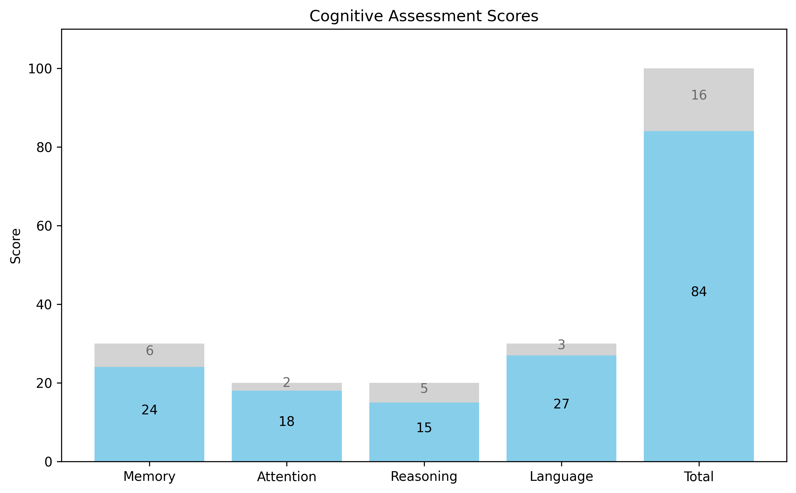
# Psychology example for addition
# Let's sum up scores from different sections of a cognitive assessment

memory_score = 24      # Out of 30 points
attention_score = 18   # Out of 20 points
reasoning_score = 15   # Out of 20 points
language_score = 27    # Out of 30 points

# Calculate total score
total_score = memory_score + attention_score + reasoning_score + language_score
max_possible = 30 + 20 + 20 + 30  # Maximum possible score

print(f"Memory Score: {memory_score}/30")
print(f"Attention Score: {attention_score}/20")
print(f"Reasoning Score: {reasoning_score}/20")
print(f"Language Score: {language_score}/30")
print(f"Total Score: {total_score}/{max_possible} ({(total_score/max_possible*100):.1f}%)")

# Visualize the scores
sections = ['Memory', 'Attention', 'Reasoning', 'Language', 'Total']
scores = [memory_score, attention_score, reasoning_score, language_score, total_score]
max_scores = [30, 20, 20, 30, 100]

plt.figure(figsize=(10, 6))

# Create a stacked bar for each section
for i in range(len(sections)):
    plt.bar(sections[i], scores[i], color='skyblue')
    plt.bar(sections[i], max_scores[i] - scores[i], bottom=scores[i], color='lightgray')

for i in range(len(sections)):
    plt.text(i, scores[i]/2, f"{scores[i]}", ha='center', color='black')
    plt.text(i, scores[i] + (max_scores[i] - scores[i])/2, f"{max_scores[i] - scores[i]}", ha='center', color='dimgray')

plt.title('Cognitive Assessment Scores')
plt.ylabel('Score')
plt.ylim(0, 110)
plt.show()
Memory Score: 24/30
Attention Score: 18/20
Reasoning Score: 15/20
Language Score: 27/30
Total Score: 84/100 (84.0%)
Subtraction (-)#
Subtraction finds the difference between two numbers.
Key things to remember:
Not commutative: \(a - b \neq b - a\) (order matters)
Can result in negative numbers when a smaller number is subtracted from a larger one
\(a - 0 = a\) (subtracting zero doesn’t change the value)
\(a - a = 0\) (subtracting a number from itself gives zero)
In psychology, subtraction is used to:
Calculate changes in scores (pre-test vs. post-test)
Find differences between groups
Determine error rates (expected - observed)
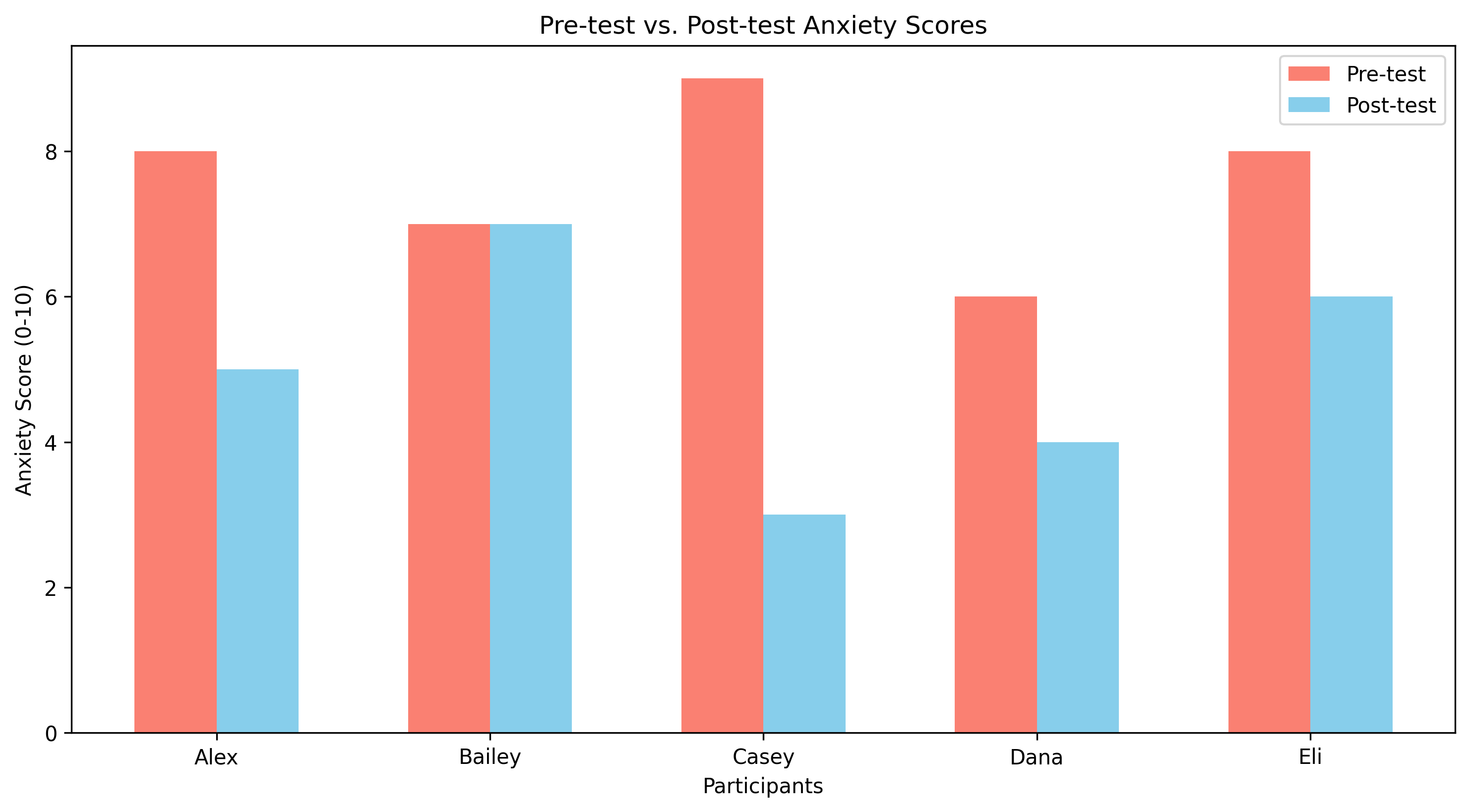
# Psychology example for subtraction
# Let's look at pre-test and post-test scores for anxiety
participants = ['Alex', 'Bailey', 'Casey', 'Dana', 'Eli']
# Anxiety scores (higher = more anxiety)
pre_test = [8, 7, 9, 6, 8] # Before therapy
post_test = [5, 7, 3, 4, 6] # After therapy
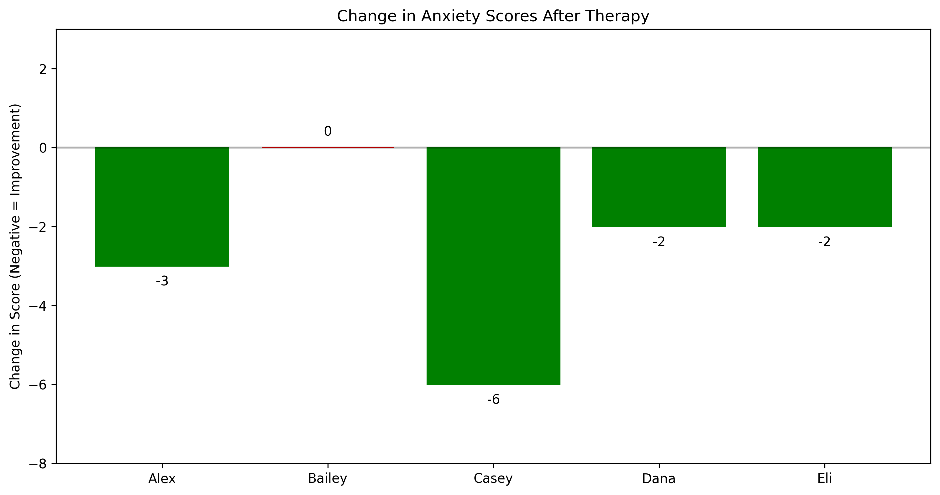
# Calculate changes (negative change means reduced anxiety, which is good)
changes = []
for i in range(len(participants)):
change = post_test[i] - pre_test[i]
changes.append(change)
# Display results
for i, name in enumerate(participants):
print(f"{name}: Pre-test {pre_test[i]}, Post-test {post_test[i]}, Change: {changes[i]}")
# Calculate average change
average_change = sum(changes) / len(changes)
print(f"\nAverage change in anxiety: {average_change:.1f}")
# Visualize the changes
plt.figure(figsize=(12, 6))
# Set width of the bars
barWidth = 0.3
# Set position of bars on X axis
r1 = np.arange(len(participants))
r2 = [x + barWidth for x in r1]
# Create bars
plt.bar(r1, pre_test, width=barWidth, color='salmon', label='Pre-test')
plt.bar(r2, post_test, width=barWidth, color='skyblue', label='Post-test')
# Add labels and legend
plt.xlabel('Participants')
plt.ylabel('Anxiety Score (0-10)')
plt.title('Pre-test vs. Post-test Anxiety Scores')
plt.xticks([r + barWidth/2 for r in range(len(participants))], participants)
plt.legend()
# Add a second plot to show the changes
plt.figure(figsize=(12, 6))
bars = plt.bar(participants, changes)
# Color bars based on whether change is positive or negative
for i, bar in enumerate(bars):
if changes[i] < 0:
bar.set_color('green') # green for improvement (reduced anxiety)
else:
bar.set_color('red') # red for worsening (increased anxiety)
plt.axhline(y=0, color='black', linestyle='-', alpha=0.3) # Add line at zero
plt.title('Change in Anxiety Scores After Therapy')
plt.ylabel('Change in Score (Negative = Improvement)')
plt.ylim(-8, 3) # Set y-axis limits
# Add value labels on top of each bar
for i, v in enumerate(changes):
if v < 0:
plt.text(i, v - 0.5, str(v), ha='center')
else:
plt.text(i, v + 0.3, str(v), ha='center')
plt.show()
Alex: Pre-test 8, Post-test 5, Change: -3
Bailey: Pre-test 7, Post-test 7, Change: 0
Casey: Pre-test 9, Post-test 3, Change: -6
Dana: Pre-test 6, Post-test 4, Change: -2
Eli: Pre-test 8, Post-test 6, Change: -2

Average change in anxiety: -2.6
Multiplication (×)#
Multiplication is repeated addition. When we multiply \(a \times b\), we’re adding \(a\) to itself \(b\) times.
Key properties:
Commutative: \(a \times b = b \times a\) (order doesn’t matter)
Associative: \((a \times b) \times c = a \times (b \times c)\) (grouping doesn’t matter)
Identity: \(a \times 1 = a\) (multiplying by 1 doesn’t change the value)
Zero property: \(a \times 0 = 0\) (multiplying by 0 gives 0)
In psychology, multiplication is used to:
Scale scores (e.g., multiplying by 2 to convert to a different scale)
Calculate total scores when items have different weights
Find expected frequencies in statistical analyses
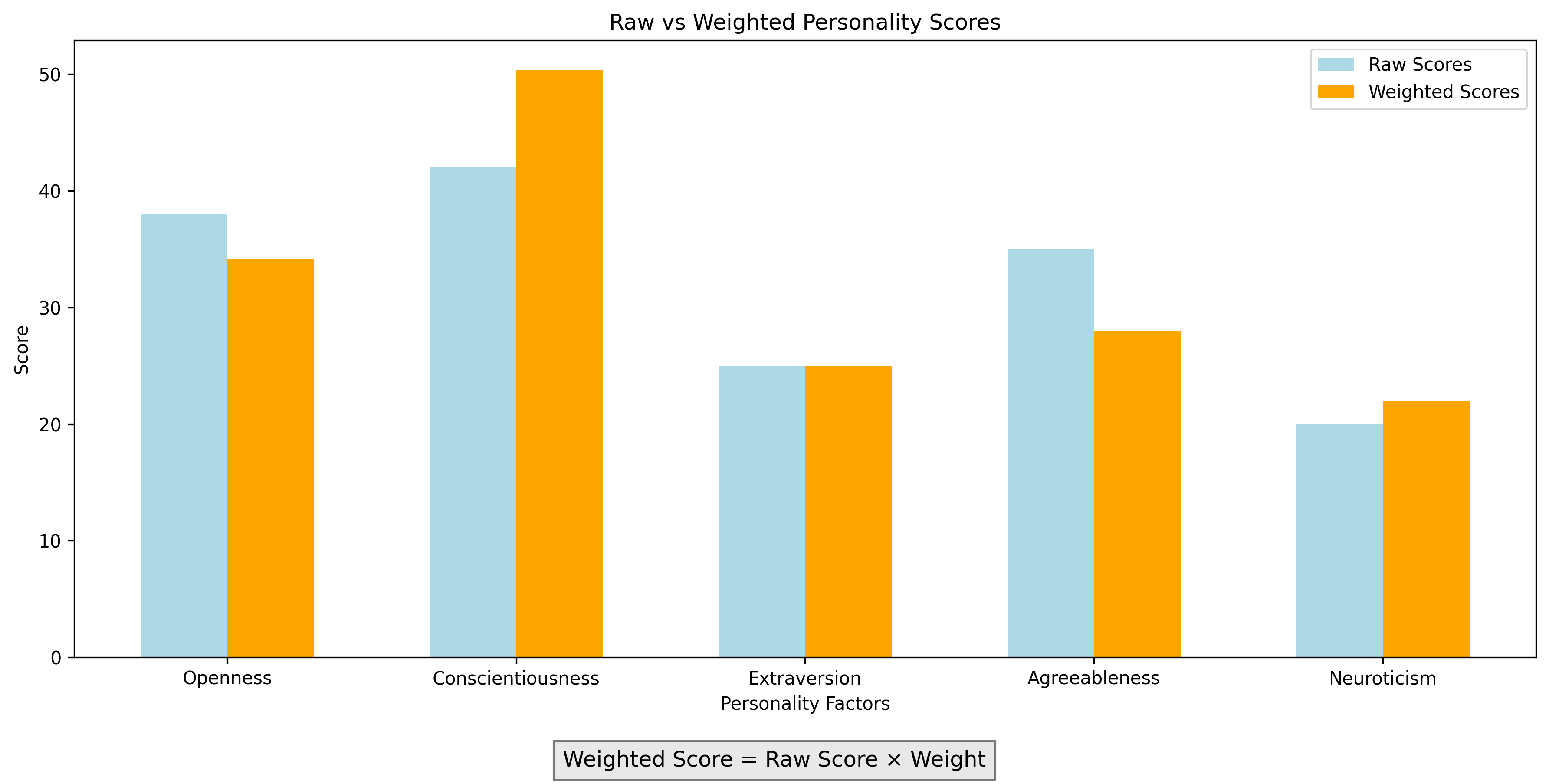
# Psychology example for multiplication
# Let's look at weighted scoring in a psychological assessment

# Personality assessment with different weights for different factors
factors = ['Openness', 'Conscientiousness', 'Extraversion', 'Agreeableness', 'Neuroticism']
raw_scores = [38, 42, 25, 35, 20]
weights = [0.9, 1.2, 1.0, 0.8, 1.1]

# Calculate weighted scores
weighted_scores = []
for i in range(len(factors)):
    weighted_score = raw_scores[i] * weights[i]
    weighted_scores.append(weighted_score)

# Display results
total_raw = sum(raw_scores)
total_weighted = sum(weighted_scores)

print("Personality Assessment Results:\n")
print(f"{'Factor':<15} {'Raw Score':<10} {'Weight':<10} {'Weighted Score':<15}")
print("-" * 50)
for i, factor in enumerate(factors):
    print(f"{factor:<15} {raw_scores[i]:<10} {weights[i]:<10} {weighted_scores[i]:<15.1f}")
print("-" * 50)
print(f"{'Total':<15} {total_raw:<10} {'N/A':<10} {total_weighted:<15.1f}")

# Visualize the raw vs weighted scores
plt.figure(figsize=(12, 6))
barWidth = 0.3
r1 = np.arange(len(factors))
r2 = [x + barWidth for x in r1]
plt.bar(r1, raw_scores, width=barWidth, color='lightblue', label='Raw Scores')
plt.bar(r2, weighted_scores, width=barWidth, color='orange', label='Weighted Scores')
plt.xlabel('Personality Factors')
plt.ylabel('Score')
plt.title('Raw vs Weighted Personality Scores')
plt.xticks([r + barWidth/2 for r in range(len(factors))], factors)
plt.legend()
plt.figtext(0.5, 0.01, "Weighted Score = Raw Score × Weight", ha="center", fontsize=12, bbox={"facecolor":"lightgray", "alpha":0.5, "pad":5})
plt.tight_layout()
plt.subplots_adjust(bottom=0.15)
plt.show()
Personality Assessment Results:

Factor          Raw Score  Weight     Weighted Score
--------------------------------------------------
Openness        38         0.9        34.2
Conscientiousness 42         1.2        50.4
Extraversion    25         1.0        25.0
Agreeableness   35         0.8        28.0
Neuroticism     20         1.1        22.0
--------------------------------------------------
Total           160        N/A        159.6