Chapter 3.3: Decimals#
Mathematics for Psychologists and Computation
Welcome to Chapter 3.3! In this chapter, we’ll explore decimals - another way to represent parts of a whole. Decimals are especially important in psychological research when reporting precise measurements and statistics.
import matplotlib.pyplot as plt
import numpy as np
import pandas as pd
from fractions import Fraction
import warnings
warnings.filterwarnings("ignore")
plt.rcParams['axes.grid'] = False  # Ensure grid is turned off
plt.rcParams['figure.dpi'] = 300
What Are Decimals?#
Decimals are a way of writing numbers that aren’t whole numbers. They use a decimal point (.) to separate the whole number part from the fractional part.
For example:
3.5 means “three and five tenths”
0.25 means “zero and twenty-five hundredths”
4.75 means “four and seventy-five hundredths”
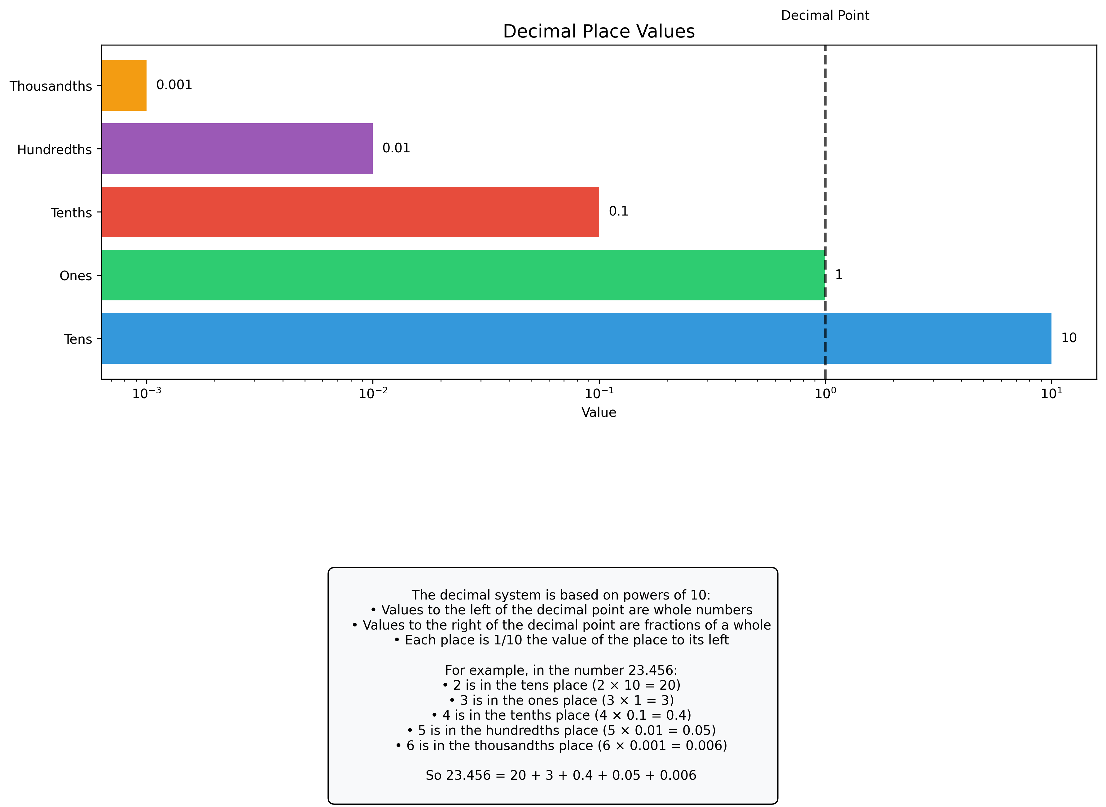
The decimal system is based on powers of 10, which gives us these place values:
Place |
Value |
|---|---|
Tens |
10 |
Ones |
1 |
Tenths |
0.1 |
Hundredths |
0.01 |
Thousandths |
0.001 |
Let’s visualize the decimal system:
# Function to visualize decimal place values
def visualize_decimal_places():
    # Create the place values and their names
    places = [10, 1, 0.1, 0.01, 0.001]
    names = ['Tens', 'Ones', 'Tenths', 'Hundredths', 'Thousandths']

    # Create a figure
    fig, ax = plt.subplots(figsize=(12, 6))

    # Create the visualization (logarithmic scale to handle different magnitudes)
    ax.barh(names, places, log=True, color=['#3498db', '#2ecc71', '#e74c3c', '#9b59b6', '#f39c12'])

    # Add values to the end of each bar
    for i, v in enumerate(places):
        ax.text(v*1.1, i, str(v), va='center')

    # Add a vertical line at x=1 to show the decimal point
    ax.axvline(x=1, color='black', linestyle='--', alpha=0.7, linewidth=2)
    ax.text(1, len(places), 'Decimal Point', ha='center', va='bottom')

    # Format the axes
    ax.set_title('Decimal Place Values', fontsize=14)
    ax.set_xlabel('Value')

    # Add an explanation
    explanation = """
    The decimal system is based on powers of 10:
    • Values to the left of the decimal point are whole numbers
    • Values to the right of the decimal point are fractions of a whole
    • Each place is 1/10 the value of the place to its left

    For example, in the number 23.456:
    • 2 is in the tens place (2 × 10 = 20)
    • 3 is in the ones place (3 × 1 = 3)
    • 4 is in the tenths place (4 × 0.1 = 0.4)
    • 5 is in the hundredths place (5 × 0.01 = 0.05)
    • 6 is in the thousandths place (6 × 0.001 = 0.006)

    So 23.456 = 20 + 3 + 0.4 + 0.05 + 0.006
    """
    plt.figtext(0.5, -0.05, explanation, ha='center', va='top',
                bbox=dict(boxstyle="round,pad=0.5", fc="#f8f9fa", ec="black", lw=1), fontsize=10)

    plt.tight_layout()
    plt.subplots_adjust(bottom=0.3)
    plt.show()

# Visualize the decimal places
visualize_decimal_places()
Converting Between Fractions and Decimals#
There are two main ways to convert between fractions and decimals:
Fraction to Decimal: Divide the numerator by the denominator
Decimal to Fraction: Express the decimal as a fraction with a power of 10 in the denominator, then simplify
Let’s look at some examples:
# Function to show fraction to decimal conversion
def fraction_to_decimal(numerator, denominator):
    decimal = numerator / denominator
    print(f"{numerator}/{denominator} = {decimal}")
    return decimal

# Show some examples
print("Converting fractions to decimals:")
examples = [(1, 4), (3, 4), (1, 3), (2, 5), (7, 8)]
for num, den in examples:
    fraction_to_decimal(num, den)

# Function to show decimal to fraction conversion
def decimal_to_fraction(decimal, display=True):
    # Use Python's Fraction class to convert and simplify
    frac = Fraction(str(decimal))
    if display:
        print(f"{decimal} = {frac.numerator}/{frac.denominator}")
    return frac

print("\nConverting decimals to fractions:")
decimal_examples = [0.25, 0.75, 0.5, 0.125, 0.625]
for dec in decimal_examples:
    decimal_to_fraction(dec)
Converting fractions to decimals:
1/4 = 0.25
3/4 = 0.75
1/3 = 0.3333333333333333
2/5 = 0.4
7/8 = 0.875

Converting decimals to fractions:
0.25 = 1/4
0.75 = 3/4
0.5 = 1/2
0.125 = 1/8
0.625 = 5/8
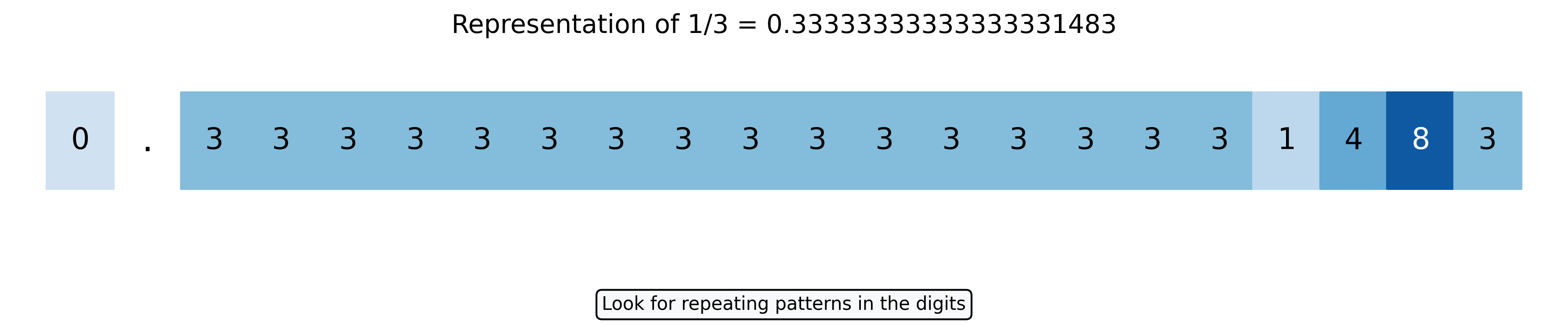
Terminating vs. Repeating Decimals#
When we convert fractions to decimals, we encounter two types:
Terminating decimals: The division ends with a remainder of zero
Example: \(\frac{1}{4} = 0.25\) (the division terminates after two decimal places)
Repeating decimals: The division never ends, with digits or groups of digits repeating forever
Example: \(\frac{1}{3} = 0.333...\) (the digit 3 repeats indefinitely)
We write this as \(0.\overline{3}\) with a bar over the repeating digit(s)
Let’s see some examples of both types:
# Examples of terminating and repeating decimals
print("Terminating decimals:")
terminating_examples = [(1, 2), (1, 4), (1, 5), (1, 8), (3, 20)]
for num, den in terminating_examples:
    decimal = num / den
    print(f"{num}/{den} = {decimal}")

print("\nRepeating decimals:")
repeating_examples = [(1, 3), (2, 3), (1, 6), (1, 7), (1, 9)]
for num, den in repeating_examples:
    # Display a longer representation to show the repetition
    decimal = num / den
    # Format to show more decimal places
    print(f"{num}/{den} = {decimal:.20f}")

# Visual representation of a repeating decimal
def visualize_repeating_decimal(num, den, decimal_places=20):
    # Calculate the decimal
    decimal = num / den
    decimal_str = f"{decimal:.{decimal_places}f}"

    # Create a figure
    plt.figure(figsize=(12, 2))

    # Plot each digit of the decimal as a colored square
    for i, digit in enumerate(decimal_str):
        if digit == '.':
            plt.text(i, 0, '.', fontsize=20, ha='center', va='center')
        else:
            # Determine color - for repeating decimals, we'll see a pattern
            color_val = int(digit) / 10
            plt.fill_between([i-0.5, i+0.5], [-0.5, -0.5], [0.5, 0.5],
                            color=plt.cm.Blues(0.2 + 0.8*color_val))
            plt.text(i, 0, digit, fontsize=16, ha='center', va='center', color='white' if int(digit) > 5 else 'black')

    # Format the plot
    plt.xlim(-1, len(decimal_str))
    plt.ylim(-1, 1)
    plt.axis('off')
    plt.title(f"Representation of {num}/{den} = {decimal_str}", fontsize=14)

    # Add annotation about repeating pattern (if any)
    if num/den != int(num/den):  # Check if it's not a whole number
        plt.figtext(0.5, -0.2, f"Look for repeating patterns in the digits",
                   ha='center', fontsize=10,
                   bbox=dict(boxstyle="round,pad=0.3", fc="#f8f9fa", ec="black", lw=1))

    plt.tight_layout()
    plt.show()

# Visualize a repeating decimal
visualize_repeating_decimal(1, 3)
Terminating decimals:
1/2 = 0.5
1/4 = 0.25
1/5 = 0.2
1/8 = 0.125
3/20 = 0.15

Repeating decimals:
1/3 = 0.33333333333333331483
2/3 = 0.66666666666666662966
1/6 = 0.16666666666666665741
1/7 = 0.14285714285714284921
1/9 = 0.11111111111111110494
Operations with Decimals#
Operations with decimals follow the same principles as operations with whole numbers, but we need to be careful with the decimal point.
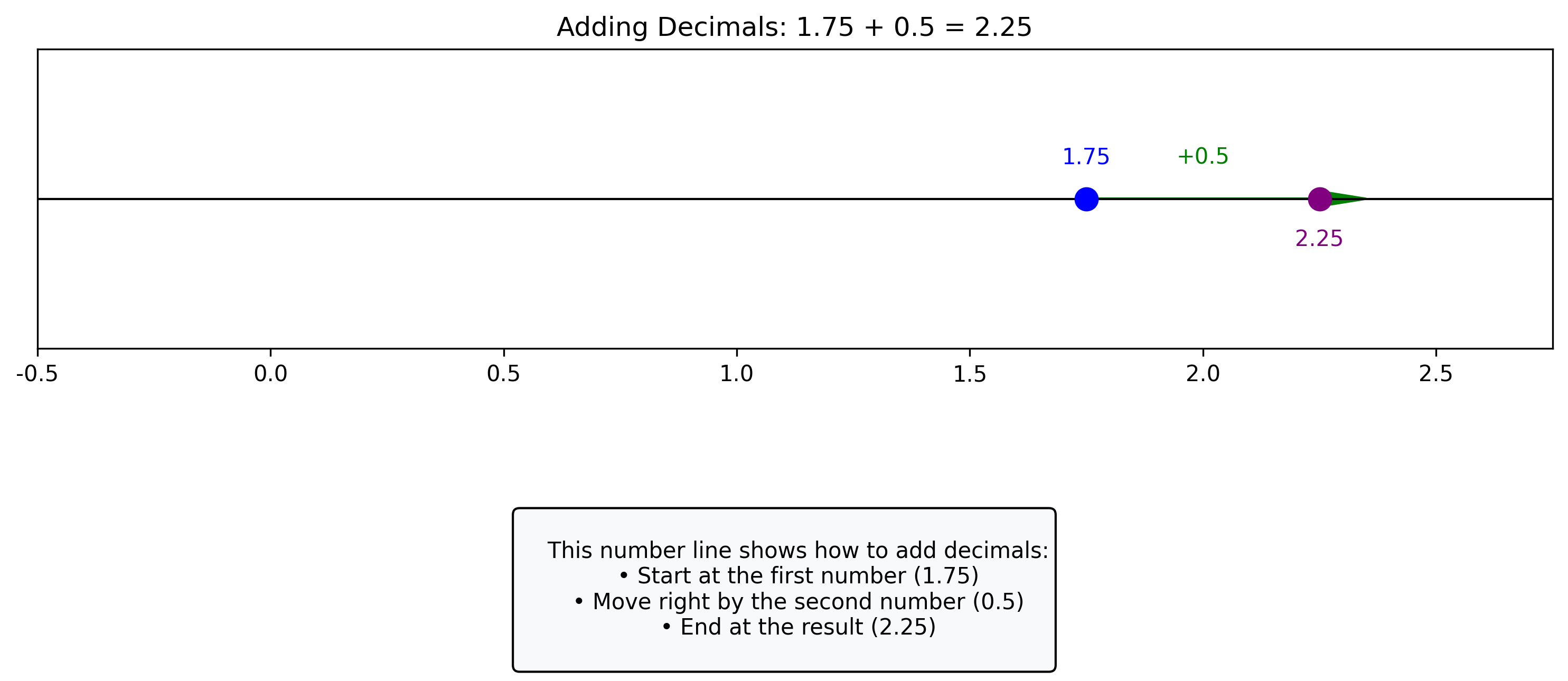
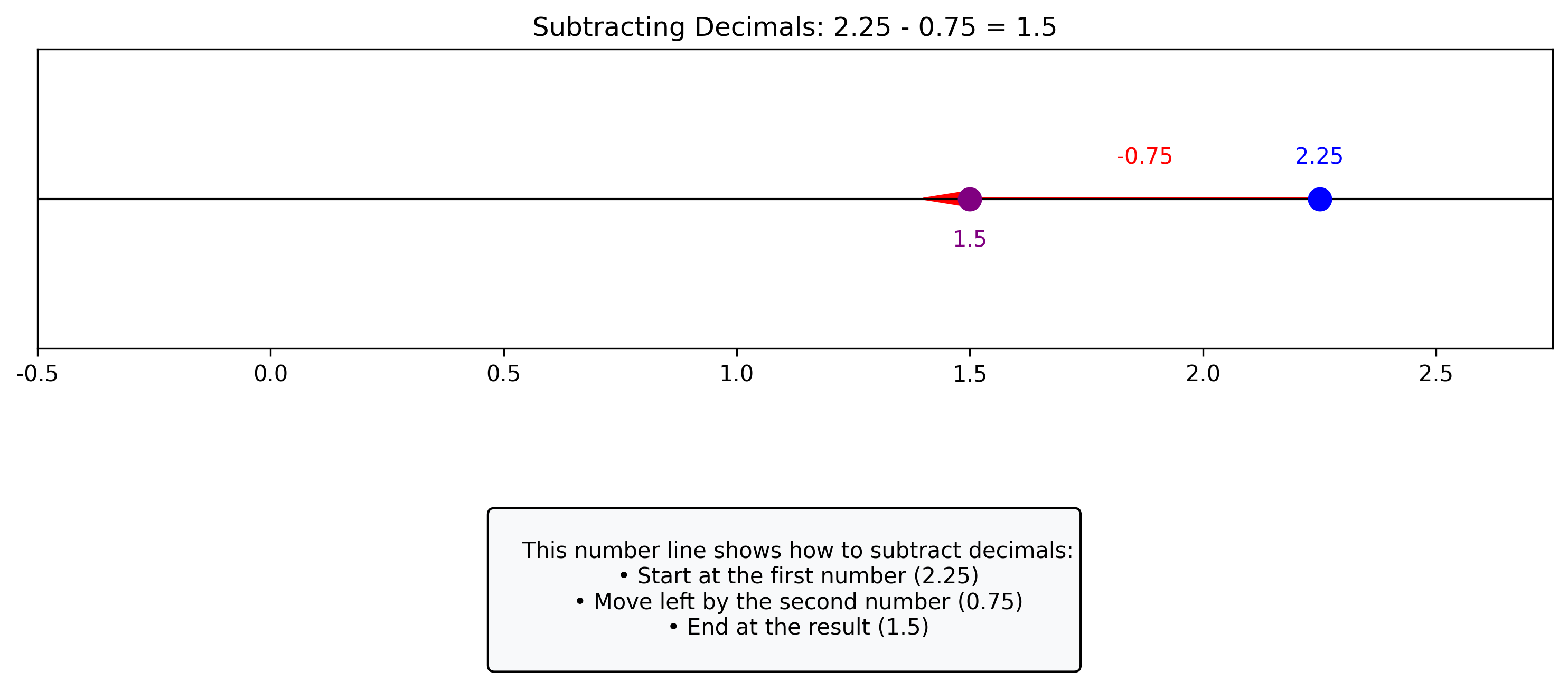
Adding and Subtracting Decimals#
When adding or subtracting decimals, we line up the decimal points to make sure we’re adding corresponding place values.
Write the numbers with the decimal points aligned
Add or subtract as with whole numbers
Keep the decimal point in the same position in the result
# Function to demonstrate decimal addition
def show_decimal_addition(a, b):
    result = a + b
    print(f"{a} + {b} = {result}")
    return result

# Function to demonstrate decimal subtraction
def show_decimal_subtraction(a, b):
    result = a - b
    print(f"{a} - {b} = {result}")
    return result

# Examples
print("Adding decimals:")
addition_examples = [(1.5, 2.75), (0.25, 0.5), (3.14, 2.86), (0.125, 0.875)]
for a, b in addition_examples:
    show_decimal_addition(a, b)

print("\nSubtracting decimals:")
subtraction_examples = [(5.75, 2.5), (1.0, 0.25), (7.3, 4.15), (1.0, 0.333)]
for a, b in subtraction_examples:
    show_decimal_subtraction(a, b)
Adding decimals:
1.5 + 2.75 = 4.25
0.25 + 0.5 = 0.75
3.14 + 2.86 = 6.0
0.125 + 0.875 = 1.0

Subtracting decimals:
5.75 - 2.5 = 3.25
1.0 - 0.25 = 0.75
7.3 - 4.15 = 3.1499999999999995
1.0 - 0.333 = 0.667
Let’s visualize decimal addition and subtraction on a number line:
# Function to visualize decimal addition on a number line
def visualize_decimal_operation(a, b, operation='addition'):
    if operation == 'addition':
        result = a + b
        op_symbol = '+'
        arrow_direction = 1  # Positive for addition
        title = f"Adding Decimals: {a} + {b} = {result}"
    else:  # subtraction
        result = a - b
        op_symbol = '-'
        arrow_direction = -1  # Negative for subtraction
        title = f"Subtracting Decimals: {a} - {b} = {result}"

    # Determine the range for the number line
    x_min = min(0, a, b, result) - 0.5
    x_max = max(a, b, result) + 0.5

    # Create the figure
    fig, ax = plt.subplots(figsize=(10, 3))

    # Draw the number line
    ax.axhline(y=0, color='black', linestyle='-', linewidth=1)

    # Add tick marks and labels
    tick_positions = np.arange(np.floor(x_min), np.ceil(x_max) + 0.1, 0.5)
    ax.set_xticks(tick_positions)
    ax.set_xticklabels([str(x) for x in tick_positions])

    # Plot the first number
    ax.plot(a, 0, 'o', markersize=10, color='blue')
    ax.text(a, 0.1, str(a), ha='center', va='bottom', color='blue')

    # Draw an arrow representing the operation
    if operation == 'addition':
        ax.arrow(a, 0, b, 0, head_width=0.05, head_length=0.1, fc='green', ec='green')
        ax.text(a + b/2, 0.1, f"+{b}", ha='center', va='bottom', color='green')
    else:  # subtraction
        ax.arrow(a, 0, -b, 0, head_width=0.05, head_length=0.1, fc='red', ec='red')
        ax.text(a - b/2, 0.1, f"-{b}", ha='center', va='bottom', color='red')

    # Plot the result
    ax.plot(result, 0, 'o', markersize=10, color='purple')
    ax.text(result, -0.1, str(result), ha='center', va='top', color='purple')

    # Format the plot
    ax.set_ylim(-0.5, 0.5)
    ax.set_xlim(x_min, x_max)
    ax.set_title(title)
    ax.set_yticks([])

    # Add an explanation
    explanation = f"""
    This number line shows how to {operation == 'addition' and 'add' or 'subtract'} decimals:
    • Start at the first number ({a})
    • Move {operation == 'addition' and 'right' or 'left'} by the second number ({b})
    • End at the result ({result})
    """
    plt.figtext(0.5, -0.1, explanation, ha='center', va='top',
                bbox=dict(boxstyle="round,pad=0.3", fc="#f8f9fa", ec="black", lw=1), fontsize=10)

    plt.tight_layout()
    plt.subplots_adjust(bottom=0.25)
    plt.show()

# Example: Visualize decimal addition
visualize_decimal_operation(1.75, 0.5, 'addition')

# Example: Visualize decimal subtraction
visualize_decimal_operation(2.25, 0.75, 'subtraction')
Multiplying Decimals#
When multiplying decimals, we follow these steps:
Multiply the numbers as if they were whole numbers, ignoring the decimal points
Count the total number of decimal places in both factors
Place the decimal point in the result so that it has that many decimal places
Let’s see some examples:
# Function to demonstrate decimal multiplication
def show_decimal_multiplication(a, b):
    result = a * b
    print(f"{a} × {b} = {result}")
    return result

# Examples
print("Multiplying decimals:")
multiplication_examples = [(1.5, 2.0), (0.5, 0.5), (2.5, 0.4), (0.25, 0.25)]
for a, b in multiplication_examples:
    show_decimal_multiplication(a, b)

# Function to explain the decimal placement in multiplication
def explain_decimal_multiplication(a, b):
    # Count decimal places
    a_str = str(a)
    b_str = str(b)
    a_decimal_places = len(a_str.split('.')[1]) if '.' in a_str else 0
    b_decimal_places = len(b_str.split('.')[1]) if '.' in b_str else 0
    total_decimal_places = a_decimal_places + b_decimal_places

    # Multiply as whole numbers
    a_whole = int(a_str.replace('.', ''))
    b_whole = int(b_str.replace('.', ''))
    result_whole = a_whole * b_whole

    # Format the result with proper decimal places
    result_str = str(result_whole)
    if total_decimal_places > 0:
        # Pad with zeros if needed
        if len(result_str) <= total_decimal_places:
            result_str = '0' * (total_decimal_places - len(result_str) + 1) + result_str
        # Insert decimal point
        result_str = result_str[:-total_decimal_places] + '.' + result_str[-total_decimal_places:]

    # Calculate actual result for comparison
    actual_result = a * b

    # Print explanation
    print(f"\nExplaining multiplication of {a} × {b}:")
    print(f"1. {a} has {a_decimal_places} decimal places")
    print(f"2. {b} has {b_decimal_places} decimal places")
    print(f"3. Total decimal places: {a_decimal_places} + {b_decimal_places} = {total_decimal_places}")
    print(f"4. Multiply as whole numbers: {a_whole} × {b_whole} = {result_whole}")
    print(f"5. Place decimal point {total_decimal_places} places from the right: {result_str}")
    print(f"6. Final result: {actual_result}")

# Example explanation
explain_decimal_multiplication(0.25, 0.5)
Multiplying decimals:
1.5 × 2.0 = 3.0
0.5 × 0.5 = 0.25
2.5 × 0.4 = 1.0
0.25 × 0.25 = 0.0625

Explaining multiplication of 0.25 × 0.5:
1. 0.25 has 2 decimal places
2. 0.5 has 1 decimal places
3. Total decimal places: 2 + 1 = 3
4. Multiply as whole numbers: 25 × 5 = 125
5. Place decimal point 3 places from the right: 0.125
6. Final result: 0.125
Dividing Decimals#
When dividing decimals, we follow these steps:
Move the decimal point in the divisor to make it a whole number
Move the decimal point in the dividend the same number of places
Divide as with whole numbers
Place the decimal point in the quotient directly above where it is in the dividend
Let’s see some examples:
# Function to demonstrate decimal division
def show_decimal_division(a, b):
    result = a / b
    print(f"{a} ÷ {b} = {result}")
    return result

# Examples
print("Dividing decimals:")
division_examples = [(1.5, 0.5), (2.5, 0.25), (0.75, 0.25), (1.0, 0.4)]
for a, b in division_examples:
    show_decimal_division(a, b)

# Function to explain the decimal placement in division
def explain_decimal_division(a, b):
    # Count decimal places in divisor
    b_str = str(b)
    b_decimal_places = len(b_str.split('.')[1]) if '.' in b_str else 0

    # Move decimal points
    b_whole = int(b_str.replace('.', '')) * (10 ** (-b_decimal_places))
    a_adjusted = a * (10 ** b_decimal_places)

    # Calculate result
    result = a / b

    # Print explanation
    print(f"\nExplaining division of {a} ÷ {b}:")
    print(f"1. The divisor {b} has {b_decimal_places} decimal places")
    print(f"2. Multiply both numbers by 10^{b_decimal_places} to make the divisor a whole number")
    print(f"3. This gives: {a_adjusted} ÷ {int(b * (10 ** b_decimal_places))}")
    print(f"4. Divide as with whole numbers: {a_adjusted} ÷ {int(b * (10 ** b_decimal_places))} = {result}")
    print(f"5. Final result: {result}")

# Example explanation
explain_decimal_division(1.5, 0.25)
Dividing decimals:
1.5 ÷ 0.5 = 3.0
2.5 ÷ 0.25 = 10.0
0.75 ÷ 0.25 = 3.0
1.0 ÷ 0.4 = 2.5

Explaining division of 1.5 ÷ 0.25:
1. The divisor 0.25 has 2 decimal places
2. Multiply both numbers by 10^2 to make the divisor a whole number
3. This gives: 150.0 ÷ 25
4. Divide as with whole numbers: 150.0 ÷ 25 = 6.0
5. Final result: 6.0
Decimals in Psychological Research#
Decimals are ubiquitous in psychological research. They’re used for:
Measurements: Reaction times (e.g., 0.523 seconds), scores on scales (e.g., 4.2 on a 5-point scale)
Statistics: Means (e.g., 3.75), standard deviations (e.g., 0.89), correlations (e.g., r = 0.42)
Proportions: Converting percentages to decimals (e.g., 75% = 0.75)
p-values: Statistical significance (e.g., p = 0.025)
Let’s create a realistic psychology example:
# Example: Analyzing reaction times in a psychology experiment

# Simulate reaction time data (in seconds) for two conditions
np.random.seed(42)  # For reproducibility

# Condition A: Standard stimulus
reaction_times_A = np.random.normal(0.450, 0.075, 20).round(3)

# Condition B: Enhanced stimulus (expected to be faster)
reaction_times_B = np.random.normal(0.375, 0.060, 20).round(3)

# Create a DataFrame to store the data
data = pd.DataFrame({
    'Condition A': reaction_times_A,
    'Condition B': reaction_times_B
})

# Calculate summary statistics
summary = data.describe().round(3)
print("Summary Statistics (reaction times in seconds):")
print(summary)

# Calculate the mean difference
mean_diff = data['Condition A'].mean() - data['Condition B'].mean()
print(f"\nMean difference (A - B): {mean_diff:.3f} seconds")

# Calculate the percentage improvement
pct_improvement = (mean_diff / data['Condition A'].mean()) * 100
print(f"Percentage improvement: {pct_improvement:.1f}%")
Summary Statistics (reaction times in seconds):
       Condition A  Condition B
count       20.000       20.000
mean         0.437        0.359
std          0.072        0.058
min          0.307        0.257
25%          0.401        0.310
50%          0.432        0.359
75%          0.488        0.387
max          0.568        0.486

Mean difference (A - B): 0.078 seconds
Percentage improvement: 17.9%
# Visualize the reaction time data
plt.figure(figsize=(10, 6))

# Create boxplots
box = plt.boxplot([reaction_times_A, reaction_times_B], labels=['Condition A', 'Condition B'],
                 patch_artist=True)

# Customize boxplot colors
colors = ['#3498db', '#e74c3c']
for patch, color in zip(box['boxes'], colors):
    patch.set_facecolor(color)

# Add individual data points (jittered for better visibility)
for i, data_points in enumerate([reaction_times_A, reaction_times_B]):
    # Create jittered x-positions
    x = np.random.normal(i+1, 0.04, size=len(data_points))
    plt.scatter(x, data_points, alpha=0.6, s=30, c='black')

# Add means as diamonds
plt.plot(1, np.mean(reaction_times_A), 'D', color='white', markersize=12, markeredgecolor='black')
plt.plot(2, np.mean(reaction_times_B), 'D', color='white', markersize=12, markeredgecolor='black')

# Label the means
plt.text(1, np.mean(reaction_times_A)+0.03, f"Mean: {np.mean(reaction_times_A):.3f}", ha='center')
plt.text(2, np.mean(reaction_times_B)+0.03, f"Mean: {np.mean(reaction_times_B):.3f}", ha='center')

# Format the plot
plt.ylabel('Reaction Time (seconds)')
plt.title('Comparison of Reaction Times Between Conditions')
plt.grid(axis='y', linestyle='--', alpha=0.7)

# Add annotation explaining the findings
plt.annotate(f"Participants responded {pct_improvement:.1f}% faster\nin Condition B compared to Condition A",
             xy=(1.5, 0.3), xytext=(1.5, 0.2),
             ha='center', va='center',
             bbox=dict(boxstyle="round,pad=0.3", fc="#f8f9fa", ec="black", lw=1))

plt.tight_layout()
plt.show()
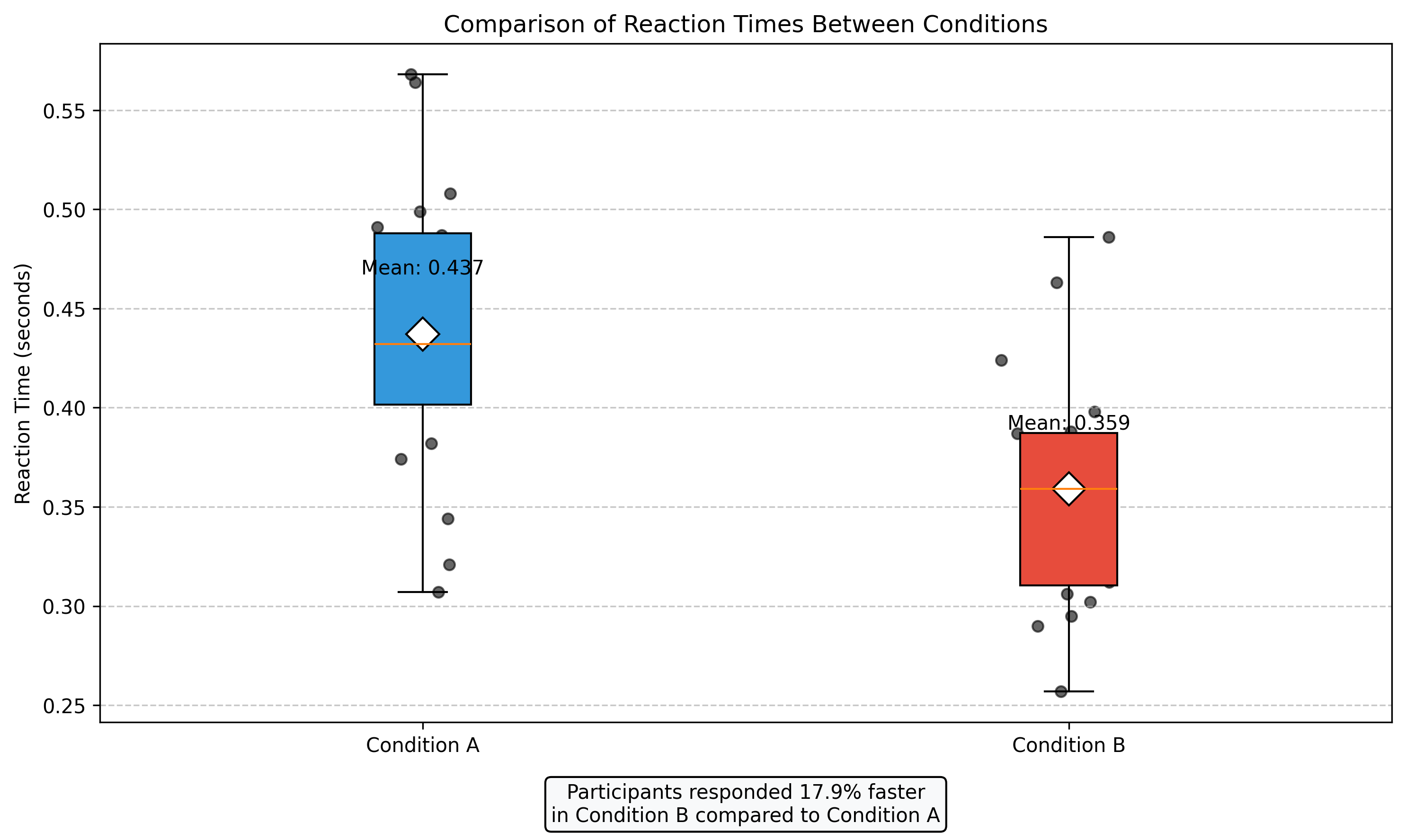
In the example above, we can see how decimals are used throughout psychological research:
Precise measurements: Reaction times measured to the millisecond (0.001 second)
Statistical summaries: Mean, standard deviation, and other statistics reported with decimal precision
Comparative analyses: Calculating differences and percentage improvements using decimal arithmetic
Visualization: Displaying decimal values in graphs for comparison and analysis
Rounding Decimals#
In psychological research, it’s often necessary to round decimals to a specific number of places. This is done for clarity, consistency, and to avoid suggesting more precision than is warranted.
Common rounding rules:
Standard rounding: Round up if the next digit is 5 or greater, otherwise round down
Reporting standards: Many disciplines have conventions about how many decimal places to report
Reaction times: typically 2-3 decimal places (e.g., 0.452 seconds)
Correlations: typically 2 decimal places (e.g., r = 0.42)
p-values: typically 3 decimal places (e.g., p = 0.023) or reported as thresholds (e.g., p < 0.05)
Let’s practice rounding decimals:
# Function to demonstrate rounding of decimals
def demonstrate_rounding(number, decimal_places):
    rounded = round(number, decimal_places)
    print(f"{number} rounded to {decimal_places} decimal places: {rounded}")
    return rounded

# Examples
print("Rounding examples:")
numbers = [3.14159, 0.6666667, 1.2345, 0.9999, 2.5000]
for num in numbers:
    for places in range(0, 4):
        demonstrate_rounding(num, places)
    print("---")

# Demonstrate psychological reporting conventions
print("\nPsychological reporting conventions:")
print("1. Reaction time: 0.4783 seconds →", round(0.4783, 3), "seconds")
print("2. Correlation coefficient: 0.6842 →", round(0.6842, 2))
print("3. p-value: 0.0349 →", round(0.0349, 3), "or p < 0.05")
print("4. Mean score on 5-point scale: 3.275 →", round(3.275, 2))
Rounding examples:
3.14159 rounded to 0 decimal places: 3.0
3.14159 rounded to 1 decimal places: 3.1
3.14159 rounded to 2 decimal places: 3.14
3.14159 rounded to 3 decimal places: 3.142
---
0.6666667 rounded to 0 decimal places: 1.0
0.6666667 rounded to 1 decimal places: 0.7
0.6666667 rounded to 2 decimal places: 0.67
0.6666667 rounded to 3 decimal places: 0.667
---
1.2345 rounded to 0 decimal places: 1.0
1.2345 rounded to 1 decimal places: 1.2
1.2345 rounded to 2 decimal places: 1.23
1.2345 rounded to 3 decimal places: 1.234
---
0.9999 rounded to 0 decimal places: 1.0
0.9999 rounded to 1 decimal places: 1.0
0.9999 rounded to 2 decimal places: 1.0
0.9999 rounded to 3 decimal places: 1.0
---
2.5 rounded to 0 decimal places: 2.0
2.5 rounded to 1 decimal places: 2.5
2.5 rounded to 2 decimal places: 2.5
2.5 rounded to 3 decimal places: 2.5
---

Psychological reporting conventions:
1. Reaction time: 0.4783 seconds → 0.478 seconds
2. Correlation coefficient: 0.6842 → 0.68
3. p-value: 0.0349 → 0.035 or p < 0.05
4. Mean score on 5-point scale: 3.275 → 3.27
Scientific Notation#
For very large or very small numbers, scientific notation is often used. This is especially common in psychology for very small p-values or effect sizes.
Scientific notation expresses a number as:
A coefficient between 1 and 10
Multiplied by a power of 10
For example:
1,500,000 = 1.5 × 10^6
0.000025 = 2.5 × 10^-5
Let’s see some examples from psychological research:
# Examples of scientific notation in psychology
examples = [
    (0.00000542, "A very small p-value"),
    (0.000000001, "Neural firing threshold (volts)"),
    (1500000, "Population size in a large-scale study"),
    (0.00000123, "Effect size for a subtle phenomenon")
]

for value, description in examples:
    scientific = "{:.2e}".format(value)  # Format in scientific notation
    print(f"{description}:")
    print(f"  Decimal: {value}")
    print(f"  Scientific notation: {scientific}")
    print("---")
A very small p-value:
  Decimal: 5.42e-06
  Scientific notation: 5.42e-06
---
Neural firing threshold (volts):
  Decimal: 1e-09
  Scientific notation: 1.00e-09
---
Population size in a large-scale study:
  Decimal: 1500000
  Scientific notation: 1.50e+06
---
Effect size for a subtle phenomenon:
  Decimal: 1.23e-06
  Scientific notation: 1.23e-06
---
Significant Figures#
Significant figures (or digits) are the meaningful digits in a number that contribute to its precision. This concept is important in scientific measurements and reporting.
Rules for identifying significant figures:
All non-zero digits are significant
Zeros between non-zero digits are significant
Leading zeros (before the first non-zero digit) are not significant
Trailing zeros after the decimal point are significant
Trailing zeros in a whole number may or may not be significant
Examples:
123.45 has 5 significant figures
0.00234 has 3 significant figures (the leading zeros are not significant)
1.200 has 4 significant figures (the trailing zeros after the decimal are significant)
1200 could have 2, 3, or 4 significant figures (ambiguous without context)
Let’s see how this applies in psychological research:
# Function to count significant figures
def count_significant_figures(number_str):
    # Convert to string if it's not already
    number_str = str(number_str)

    # Handle scientific notation
    if 'e' in number_str.lower():
        coefficient = number_str.lower().split('e')[0]
        return count_significant_figures(coefficient)

    # Remove decimal point
    number_str = number_str.replace('.', '')

    # Remove leading zeros
    number_str = number_str.lstrip('0')

    # Count the remaining digits
    return len(number_str)

# Examples from psychology
psych_examples = [
    ("0.05", "Common significance threshold"),
    ("0.001", "Stricter significance threshold"),
    ("0.732", "Correlation coefficient"),
    ("120.00", "Sample size (specified precision)"),
    ("3.14159", "Calculated statistic")
]

print("Significant figures in psychological measurements:")
for value, description in psych_examples:
    sig_figs = count_significant_figures(value)
    print(f"{description}: {value} has {sig_figs} significant figures")
Significant figures in psychological measurements:
Common significance threshold: 0.05 has 1 significant figures
Stricter significance threshold: 0.001 has 1 significant figures
Correlation coefficient: 0.732 has 3 significant figures
Sample size (specified precision): 120.00 has 5 significant figures
Calculated statistic: 3.14159 has 6 significant figures
Using Decimals in Python for Psychological Data Analysis#
Python provides several ways to work with decimals in data analysis, which is particularly useful for psychological research:
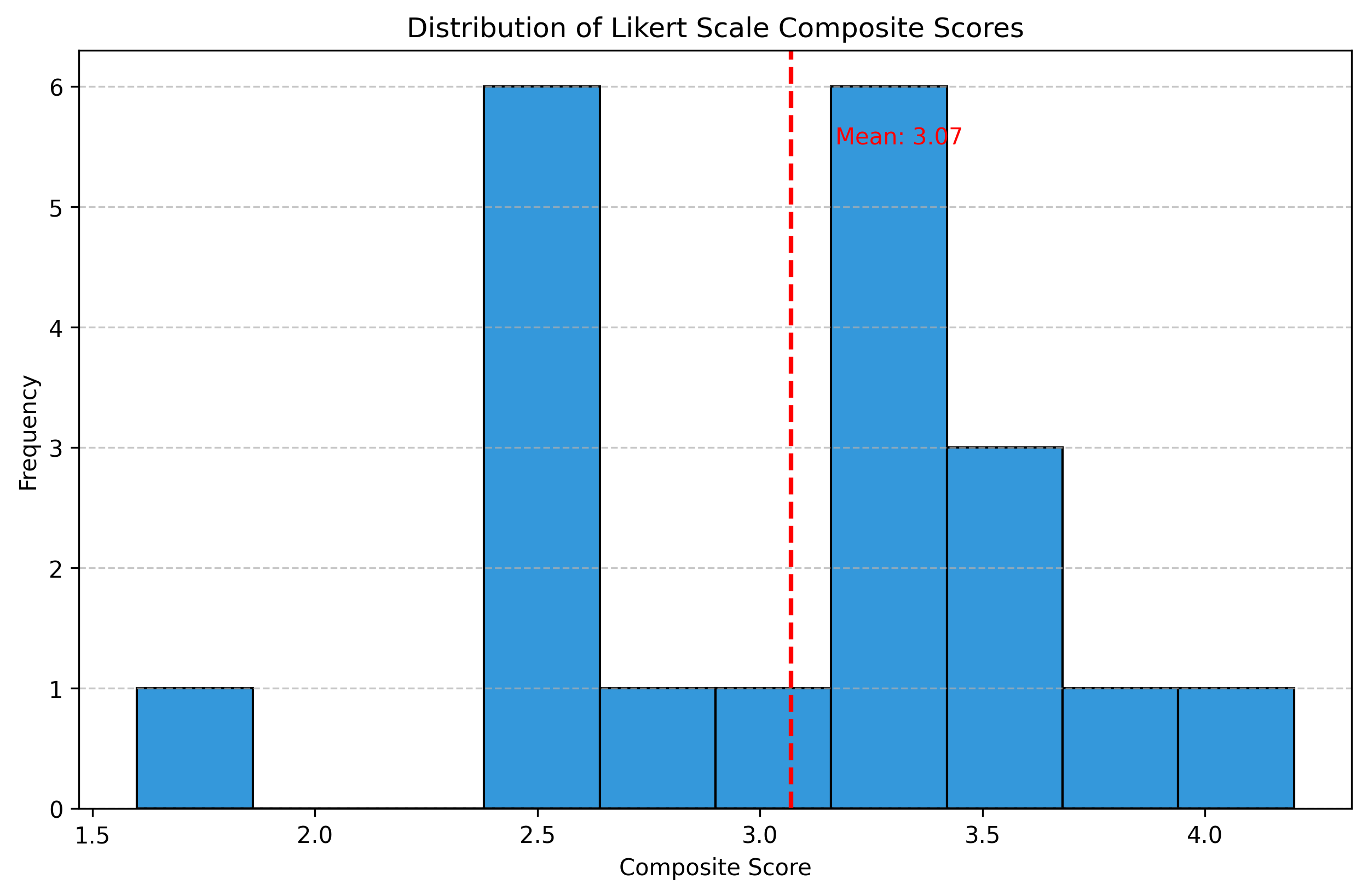
# Example: Analyzing Likert scale responses
# Likert scales are commonly used in psychology (e.g., 1=Strongly Disagree to 5=Strongly Agree)

# Simulate responses from 20 participants on 5 questions
np.random.seed(123)
likert_responses = np.random.randint(1, 6, size=(20, 5))

# Create a DataFrame
likert_df = pd.DataFrame(likert_responses,
                         columns=['Q1', 'Q2', 'Q3', 'Q4', 'Q5'])

# Calculate mean and standard deviation for each question
question_stats = likert_df.describe().loc[['mean', 'std']].round(2)
print("Likert scale responses (1-5):")
print(question_stats)

# Calculate composite score (average across all questions)
likert_df['Composite'] = likert_df.mean(axis=1).round(2)

# Visualize the distribution of composite scores
plt.figure(figsize=(10, 6))
plt.hist(likert_df['Composite'], bins=10, color='#3498db', edgecolor='black')
plt.axvline(likert_df['Composite'].mean(), color='red', linestyle='--', linewidth=2)
plt.text(likert_df['Composite'].mean() + 0.1, plt.ylim()[1]*0.9,
         f"Mean: {likert_df['Composite'].mean():.2f}",
         color='red', va='top')

plt.xlabel('Composite Score')
plt.ylabel('Frequency')
plt.title('Distribution of Likert Scale Composite Scores')
plt.grid(axis='y', linestyle='--', alpha=0.7)
plt.show()
Likert scale responses (1-5):
        Q1    Q2    Q3    Q4    Q5
mean  3.65  3.25  2.90  2.50  3.05
std   1.27  1.37  1.48  1.32  1.23
Summary#
In this chapter, we’ve explored decimals and their importance in psychological research:
Decimal Basics: Understanding place values and decimal notation
Converting Between Fractions and Decimals: Methods for conversion and identifying terminating vs. repeating decimals
Operations with Decimals: Addition, subtraction, multiplication, and division
Rounding and Precision: How to round decimals and the concept of significant figures
Scientific Notation: Representing very large or small numbers
Applications in Psychology: Using decimals for measurements, statistics, and data analysis
Decimals are essential for precise measurement and analysis in psychological research, allowing researchers to capture and communicate nuanced findings.
Practice Exercises#
Convert the following fractions to decimals:
\(\frac{3}{8}\)
\(\frac{2}{3}\)
\(\frac{5}{16}\)
\(\frac{7}{20}\)
Convert the following decimals to fractions in simplest form:
0.75
0.125
0.6
0.35
Perform the following operations:
0.75 + 0.25
1.5 - 0.75
0.2 × 0.5
0.8 ÷ 0.2
Round the following numbers to the indicated decimal places:
3.14159 to 2 decimal places
0.6666667 to 3 decimal places
42.999 to 1 decimal place
0.055555 to 2 decimal places
Psychological Application: A psychologist recorded the following reaction times (in seconds) for a participant across 5 trials: 0.423, 0.456, 0.387, 0.412, 0.442. Calculate:
The mean reaction time
The fastest and slowest times
The difference between the fastest and slowest times
The percentage improvement from the slowest to the fastest time
Python Challenge: Use the techniques from this chapter to analyze a set of test scores [87.5, 92.3, 78.6, 85.4, 91.7, 76.3, 89.2, 84.5, 93.8, 79.1]. Calculate the mean score, convert it to a fraction in simplest form, and create a visualization showing each score’s deviation from the mean.